Programming in R – From Variables to Visualizations

This article was published as a part of the Data Science Blogathon

R programing language was developed for statistical computing and graphics which makes it one of the desired candidates for Data Science and Analysis. Even though it might not hold much popularity among the newcomers in the field, many veterans and seasoned data scientists favour R over Python.

Though opinions might vary from individual to individual, here is a nice article comparing the key differences between the languages and discusses why there’s this ongoing war for the title of Best programming language for Data Science:

R or Python? Reasons behind this Cloud War | Shankar_DK

Though I am nowhere near as qualified to comment on this subject, I’d like to say that every beginner shall try both the languages and decide for themselves what they want, rather than following the crowd. Following my own advice, I recently started learning R as my semester has ended and I had nothing better to do, and thought of sharing my learning path with my readers.

As I said, I am learning R for the first time myself so if there are any mistakes, or improvements, or some suggestions, I’d love to hear from you guys in the comment section below. I’m sure this tutorial will be very helpful for my beginner readers, so let’s get started!

Datasets used:

1. Titanic- Machine Learning from Disaster

2. Iris species

3. House Prices – Advanced Regression techniques

Table of contents

1) Introduction

2) Variables and Assignment

3) Data Structures

• Vector
• Arrays and Matrices
• Lists
• Factors
• DataFrames

4) Indexing, Slicing, and Striding

• Vectors and Matrices
• Lists and DataFrames

5) Importing Data

6) Control Statements

• statement
• The If/else If/else statement
• While loop
• next and break statement
• For loop
• Nested for loop

7) Functions

8) DataFrame manipulation using dplyr

• select()
• filter()
• arrange()
• rename()
• mutate()

9) Plotting with R

• Histogram
• Boxplot
• Scatterplot
• Line Plot
• Barplot
• Pie Chart

10) Visualization using ggplot2

• Scatterplot
• Histogram
• Boxplot
• Barplot
• Density Plot
• Violin Plot
• Pie Chart
• Line Plot
• Maps

11) Correlation heatmap using corrplot

12) Endnoted

Introduction

R is a programming language as well as a free statistical computing environment. It was released in 1993 and is a dialect of the S programming language. Just like Python, R has around 13000 library packages for Data Analysis, Statistical Methods, and visualizations. Read the official docs for more details, and now time for the technical and exciting stuff!

Variables and Assignment in R

In R the assignment operator is <-

x <- 21    # assign the value 5 to variable x 
x          # print the value of x

output:

21

We use parenthesis () to assign a value and print it at the same time.

(y <- 5)  # assigning value 5 to the variable y and printing its value

output:

5

Data Structures in R

Just like any other programming language, R has its containers called data types to store values or information. R has 5 primary data types:

1. integers
2. doubles
3. logical
4. characters
5. complex

Apart from these, there are secondary data types in R, which are more useful and commonly used

• Vector: sequence of primary data types
• Arrays and Matrices: a multi-dimensional collection of homogenous vectors
• Lists: vectors with either homogeneous or heterogeneous type(i.e can contain different or similar types of basic data types)
• Factors: categorical or ordinal data
• Data Frame: multi-dimensional array of possible heterogeneous data types

Let’s look into some examples of these secondary data types:

1) Vector

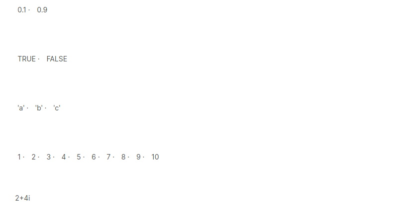
It is a sequence of similar data types. The concatenate function c() can be used to join data to create vectors. Simple sequences can be created using the colon ‘:’ operator.

a <- c(0.1, 0.9)       # numeric
a
b <- c(TRUE, FALSE)    # logical
b
d <- c("a", "b", "c")  # character
d
e <- 1:10              # integer
e
f <- c(2+4i)           # complex
f

output:

The seq() function can also be used to create a vector with a specific sequence. This function also accepts a stepsize of default value 1.

# A sequence of numbers from 1 to 10 with a step size of 1. 
seq(1, 10)

output:

# A sequence of numbers in step size of 2
seq(0, 20, by=2)

output:

# A sequence of numbers from 10 to 20 of length 5 (they are equally spaced)
seq(10, 20, len=5)

output:

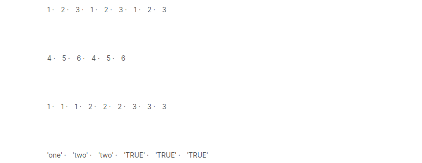
The rep() function is used to create a vector by replicating specified values

rep(1:3, times=3)                       # repeat (1,2,3) 3x
rep(4:6, 2)                             # repeat (4,5,6) 2x
rep(1:3, each=3)                        # repeat each of (1,2,3) 3x
rep(c('one', 'two', 'TRUE'), times=1:3) # repeat ('one', 'two', 'TRUE') frist element 1x, second element 2x and third element 3x

output:

2) Arrays and Matrices

The function array() is used for creating arrays and matrix() for matrices. Arrays can be converted into matrices by changing the dim() attribute.

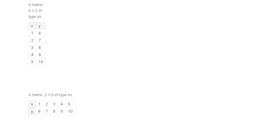
Row or column matrices can be created using rbind() and cbind() functions.

mat <- matrix(1:12, nrow=3, ncol=4)
mat

dim(mat)

output:

arr <- array(1:12)
arr

output:

dim(arr) <- c(3,4)
arr

output: 

x <- 1:5
y <- 6:10

cbind(x, y)
rbind(x, y)

output:

3) Lists

Just like python lists, the lists in R are heterogeneous containers and are created using the list() function.

L <- list(10, 'name', TRUE, 0.5)
L

output:

1. 10
2. ‘name’
3. TRUE
4. 0.5

l <- list(x=1:3, y=c('a', 'b', 'c'), z=c(T, F, F))
l

output:

4) Factors

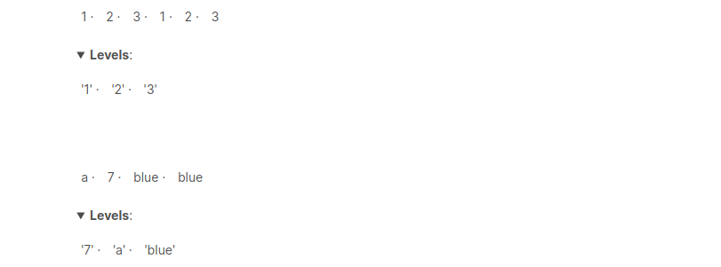
Categorical and ordinal data is represented using factors in R using the factor() function. Factor levels contain all the possible values the elements can take.

f1 <- factor(rep(1:3, times=2))
f1
f2 <- factor(c('a', 7, 'blue', 'blue'))
f2

output:

x <- factor(c("True", "False", "False", "True", "True"),
            levels = c("False", "True"))
x

output: 

z <- factor(
    c("Thr", "Thr", "Fri", "Thr", "Wed", "Wed", "Mon", "Tue"),
    levels = c("Mon", "Tue", "Wed", "Thr", "Fri"),
    ordered = TRUE
    )
z

output:

factor(c("H", "H", "T", "H", "T"))

table(factor(c("H", "H", "T", "H", "T")))

output:

5) Data Frames

unlike Python, R has an inbuilt DataFrame container and works similar to the one in Pandas. We use the data.frame() function where the arguments are vectors :

d <- c(1,2,3,4)
e <- c('red', 'yellow', 'green', NA)
f <- c(TRUE, TRUE, FALSE, TRUE)

mydataframe <- data.frame(d,e,f)
mydataframe

output:

We can edit the names of the column using the names() function:

names(mydataframe) <- c("ID", "Color", "Passed")

mydataframe

output:

Or you can include the name at the time of data frame creation:

dataframe3 <- data.frame(Age=c(50,35,71), 
                  Name=c('Joe', 'April', 'Brown'), 
                  Passed=c(TRUE, FALSE, TRUE))
dataframe3

output:

We can access the individual columns (vectors) using the $ sign and the name of the vector:

# getting the 'Color' vector from the DataFrame
mydataframe$Color

output:

‘red’ . ‘yellow’ . ‘green’ . NA

Indexing, Slicing, and Striding in R

For indexing or selecting elements we use [, [[, or the $ operator.

1) Vectors and Matrices

we can essentially put 4 kinds of values in the bracket [

• a vector of positive integers, in which case the specified elements are extracted,
• a vector of negative integers, where those elements are removed,
• a logical operator of the same length as the vector in question returns a boolean, or
• a character vector, where elements are extracted

x  10                # returns logical (T/F) if the element of x is greater than 10
x[x>10]               # extract elements of x which are greater than 10

output:

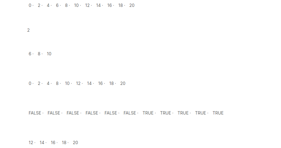
x <- 1:5                                 # assign a sequence of 0 to 20 in steps of 2 to variable x
names(x) <- c("a", "b", "c", "d", "e")   # assign names to vector x
x                                        # print x
x[c("a","c","e")]                        # extract parts of vector x by names

output:

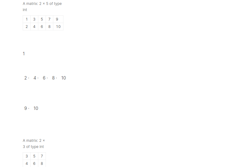
Similar indexing can be done on matrices and arrays. Here the commas are used to specify the dimension:

a <- 1:10          # array
dim(a) <- c(2, 5)  # make it a matrix

a

a[1,1]             # extract element of matrix a at row=1, col=1
a[2, ]             # extract the second row of matrix a
a[, 5]             # extract the fifth columns of matrix a (all rows)
a[, 2:4]           # extract columns 2 to 4 of matrix a (all rows)

output:

2) Lists and DataFrame

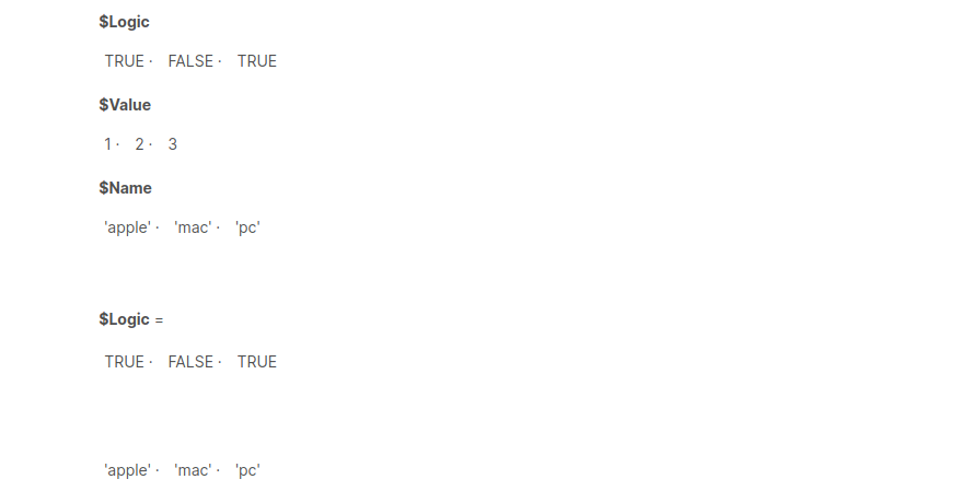
While using lists and DF we use [[ and $ too.

mylist <- list(Logic = c(TRUE, FALSE, TRUE), Value = 1:3, Name = c("apple", "mac", "pc"))

mylist        # print the list 

mylist[1]     # print the 1st element of the list

mylist$Name   # printing using names

output:

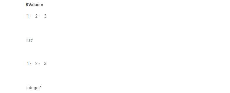
mylist[2]              # extracting the second element of mylist

typeof(mylist[2])      # checking the type of mylist[2]

mylist[[2]]            # values of mylist[2]

typeof(mylist[[2]])    # type of mylist[2]

output:

Importing Data in R

1. The read.table() function is used to import tabular data as a data frame.

2. format – read.table( file_path , header = True, sep=” , ” )

3. header = True tells R that the data has a name for the columns and thus uses the first row in the file as the column names. False is the default value if not specified, then the program will assume the file has no header.

4. sep specifies the delimiter used in the source file, for example, .csv files are used for storing data in Kaggle, thus we shall use the comma ” , ” as the delimiter for loading the data for our code below.

Example: Importing the Iris dataset, and view the first 5 entries:

path_iris = '../input/iris/Iris.csv'
iris <- read.table(file=path_iris, header= TRUE, sep =',')
iris[1:5, ]

output:

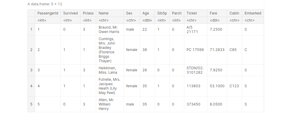
Importing Titanic dataset and view the first 5 entries:

path_titanic = '../input/titanic/train.csv'
titanic <- read.table(file=path_titanic, header= TRUE, sep =',')
titanic[1:5, ]

output:

Control statements

Controloll statements allow us to introduce logic into our codes. The statements like If, If else and loops run similar to that of Python, so this section might be simpler for those who are already familiar with it.

1) If() statement

Syntax:

if (Condition)

{ Statement }

The {statement} part of the code is executed only if the {condition} part of the If statement is satisfied. If the condition is not satisfied, the R interpreter skips that segment of the code.

Example:

if (1 == 1) {
print("yes!!")
}

output:

yes!!

Note:

• The if() statement can only check a single element, not a vector. If applied to a vector, will only check if the first element satisfies the condition.
• If the first element does not satisfy the condition, none of the statements will be executed, and a non-fatal warning will be issued indicating that the body of the if() statement is not executed. any() or all() function shall be used to check the truth on a vector.
• For single-lined statements, the curly braces can be omitted but it is good practice to keep them.

Example:

x =5) {x^2}

x 0)) {x^2}

x =10)) {x^2}

output:

2) The If/else If/else statement

Syntax:

if (Condition) { Statement }

else if { Statement }

else { Statement }

(x <- runif(1, 0, 10))           # draw a random number from a uniform dist b/w 0 nd 1

if(x < 3) {                      # if x <3 assign value 10 to variable y
        y  3 && x < 6) {     # else if x in between 3 and 6, assign value 0 to variable y
        y <- 0
} else {                         # else assign -10 to variable y
       y <- -10
}

y

output:

2.79287837212905
10

3) While loop

A while loop starts by checking a condition. If met, the loop begins and all the statements inside the body are executed. Once the body ends, the condition is checked again, and if satisfied the loop continues.

Syntax:

i = 0

while (i<5) {

print(i^2)

i = i + 1

}

i = 0                     # initialize i 
while (i < 10){           # while i = 10
}

output:

[1] "hello"
[1] "hello"
[1] "hello"
[1] "hello"
[1] "hello"
[1] "hello"
[1] "hello"
[1] "hello"
[1] "hello"
[1] "hello"

4) next and break statement

• next is used to skip a single iteration of any loop
• break is used to exit the loop then and there

# Skipping the first 5 iterations

for(i in 1:10) {
        if(i <= 5) {
                next                
        }
    print(i^2)             
}

output:

[1] 36
[1] 49
[1] 64
[1] 81
[1] 100

# print i until 5 and stop the loop

for(i in 1:10) {
      print(i) 
    if(i > 5) {
        break  
      }
}

output:

[1] 1
[1] 2
[1] 3
[1] 4
[1] 5
[1] 6

5) For loop

For loops have a predetermined number of iterations and use a variable to do so. Mostly used for iterating over iterable objects just like python.

Syntax:

for (iterator) {
Statement }

for (i in 1:5){
    print(i + 1)
}

output:

[1] 2
[1] 3
[1] 4
[1] 5
[1] 6

The seq_along() function is analogous to the len() function in python, used to generate an integer sequence based on the length of the iterator.

output:

[1] "mon"
[1] "tue"
[1] "wed"
[1] "thu"
[1] "fri"
[1] "sat"
[1] "sun"

6) Nested for loops

• Nested for loops are used to work with higher dimensional objects like lists or matrices.
• But too much nesting can ruin the readability of the code, so it is commonly advised to keep the number of nests to 2-3 max.

x <- matrix(1:6, 2, 3)

for(i in seq_len(nrow(x))) {
        for(j in seq_len(ncol(x))) {
                print(x[i, j])
        }   
}

output:

[1] 1
[1] 3
[1] 5
[1] 2
[1] 4
[1] 6

Functions

Functions are a bundle of commands used to achieve a specific outcome. They are usually used to reduce redundancy in code.

The syntax of creating a function in R is:

myfunction <- function(arg1, arg2)
{
code to execute
}

The name of this function is myfunction and accepts 2 arguments. Functions can either execute some instructions or can be used to return values. To use the function, we simply type:

myfunction(var1, var2)

Example 1:

Let us create a function using the Pythagoras theorem. The theorem states that “The square of the length of the hypotenuse of a right-angled triangle is equal to the sum of the squares of length of the other two sides.”

Where a, b, and c are the sides of the right-angled triangle. Now let’s create a function to find the hypotenuse when the sides are given:

pyth <- function(x, y)
    {
    return(sqrt((x)^2 +(y)^2))
}

pyth(3, 4)

output:

5

Example 2:

Let’s write a function to calculate the standard deviation of all the elements in a vector.

stdev <- function(x)
    {
    s <- sqrt(sum((x - mean(x))^2)/(length(x)-1))
    s
}

z <- rnorm(20)
stdev(z)

output:

1.0321309737329

DataFrame manipulation using dplyr in R

In the previous article, we learned how to import structured data in the form of DataFrame to our notebook using base R. In this section, we will learn how to manipulate this data for drawing out inferences and making visualizations.

dplyr can be thought of as the pandas of R. There’s a lot one can do with a DataFrame, and it becomes hectic to do it in native R, that’s where dplyr comes in. It has a set of ‘verbs’, a term coined by themselves, that’ll help the user to solve most of the common manipulation challenges. Some of these ‘verbs’ are:

• select()   -  selects variables according to their names
• filter()   -  selects cases according to their values
• arrange()  -   reorders rows
• mutate()   -   adds and preserves an existing variable
• summarise()-  creates a summary value from multiple values
• group_by() -  helps in performing batch operations on groups

Now we’ll demonstrate the uses of the above ‘verbs’

# importing library
library(dplyr)

importing the data:

path_iris = '../input/iris/Iris.csv'
iris <- read.table(file=path_iris, header= TRUE, sep =',')
iris[1:5, ]

path_titanic = '../input/titanic/train.csv'
titanic <- read.table(file=path_titanic, header= TRUE, sep =',')
titanic[1:5, ]

output:

 

 

1. select()

data(iris)
names(iris)[1:3]       # extract the first three columns of the iris dataset

output:

‘Sepal.Length’ . ‘Sepal.Width’ . ‘Petal.Length’

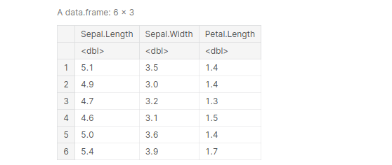
df <- select(iris, Sepal.Length:Petal.Length)
head(df)

output:

we use the ‘ – ‘ sign inside select() to omit variables we don’t want.

df <- select(iris, -(Species))
head(df, 3)

output:

Another amazing feature of select() is that it allows us to select rows based on certain patterns. This is done using “starts_with”() and “ends_with”()

df_sepal <- select(iris, "starts_with"('Sepal'))
head(df_sepal, 3)

2. filter()

Just like select() was used to extract columns, filter() is used to extract rows of the DataFrame. It is similar to the subset() function in native R.

# filter the observations with sepal length more thahn 6cm
iris_filt  6.0)
str(iris_filt)

output:

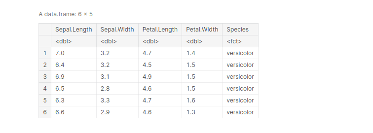
data(iris)
iris_filt  6.0 & Petal.Length < 6.0 )
head(iris_filt)

output:

3. arrange()

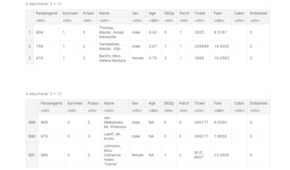
This function is used to reorder the DataFrame according to a particular column. The default is ascending order. Let’s reorder our titanic DataFrame according to age, from youngest to oldest.

titanic_age_arraned <- arrange(titanic, Age)
head(titanic_age_arraned, 3)
tail(titanic_age_arraned, 3)

output:

4. rename()

The rename() function is used to change the column names. the syntax is :

dataframe <- rename( dataframe, ‘new_name_1′ = old_name_1’ , ‘new_name_2’ = old_name_2’….)

here’s an example:

head(iris, 3)

output:

iris <- rename(iris, 'sepal_length_[cm]'= Sepal.Length, 'sepal_width_[cm]'=Sepal.Width,
               'petal_length_[cm]'=Petal.Length, 'petal_width_[cm]'=Petal.Width )
head(iris, 3)

output:

5. mutate()

mutate() is used to derive a new column from an existing column, without changing the parent column. For example, let’s create a new column in the Iris dataframe that shows the length-to-width ratio of petals and sepals of all the entries.

data(iris)
iris <-  mutate(iris, 'Petal_L2W_ratio' = Petal.Length/Petal.Width,
                      'Sepal_L2W_ratio' = Sepal.Length/Sepal.Width)
head(iris, )

output:

There’s a similar function, transmute() which essentially does the same thing as mutate(), but drops all columns that remain non-transformed :

iris <- transmute(iris, 'Petal_L2W_ratio' = Petal.Length/Petal.Width,
                      'Sepal_L2W_ratio' = Sepal.Length/Sepal.Width)
head(iris, 3)

output:

Plotting with R

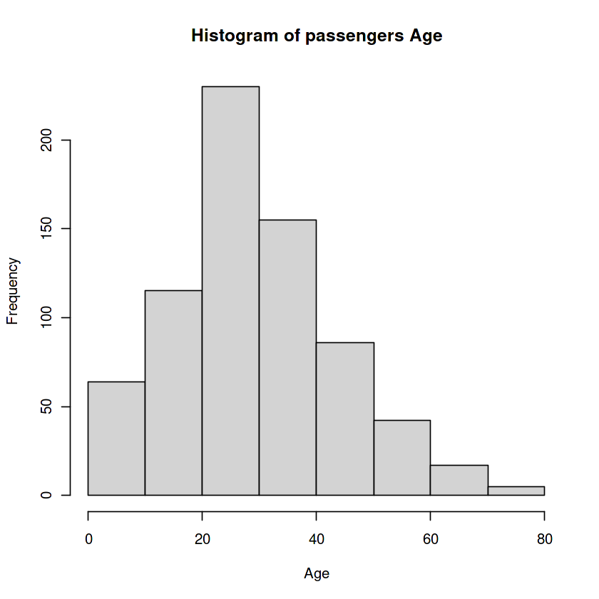
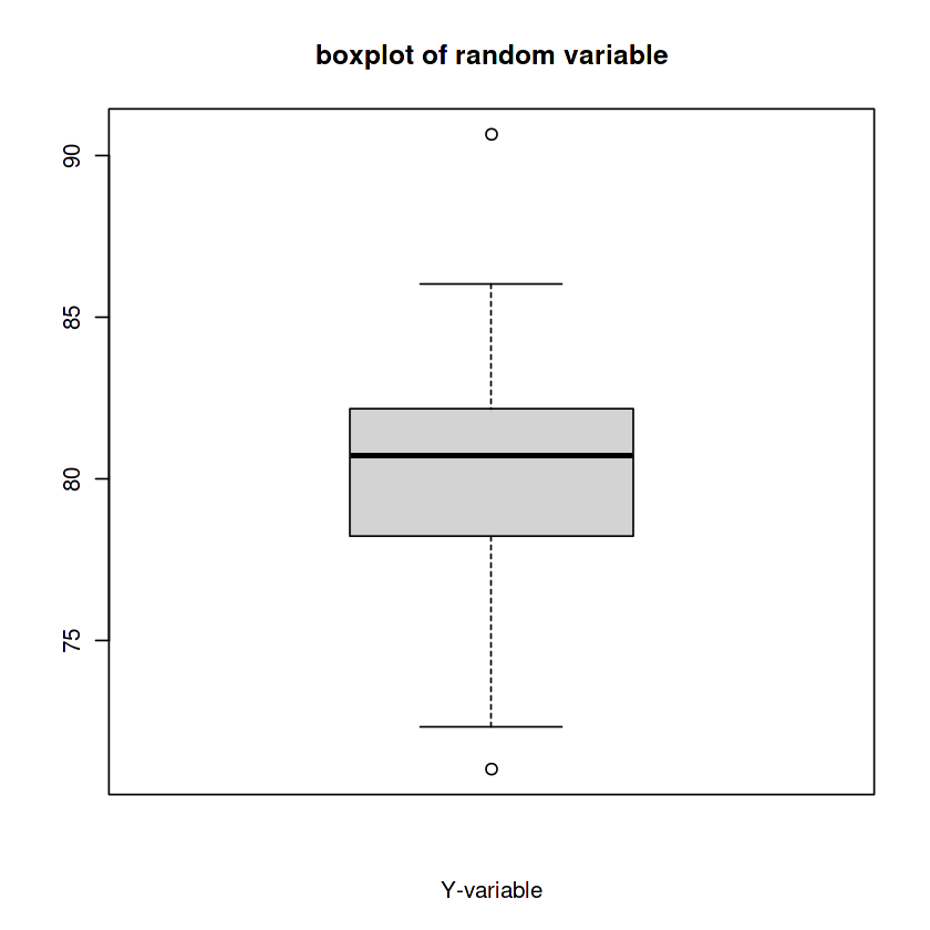
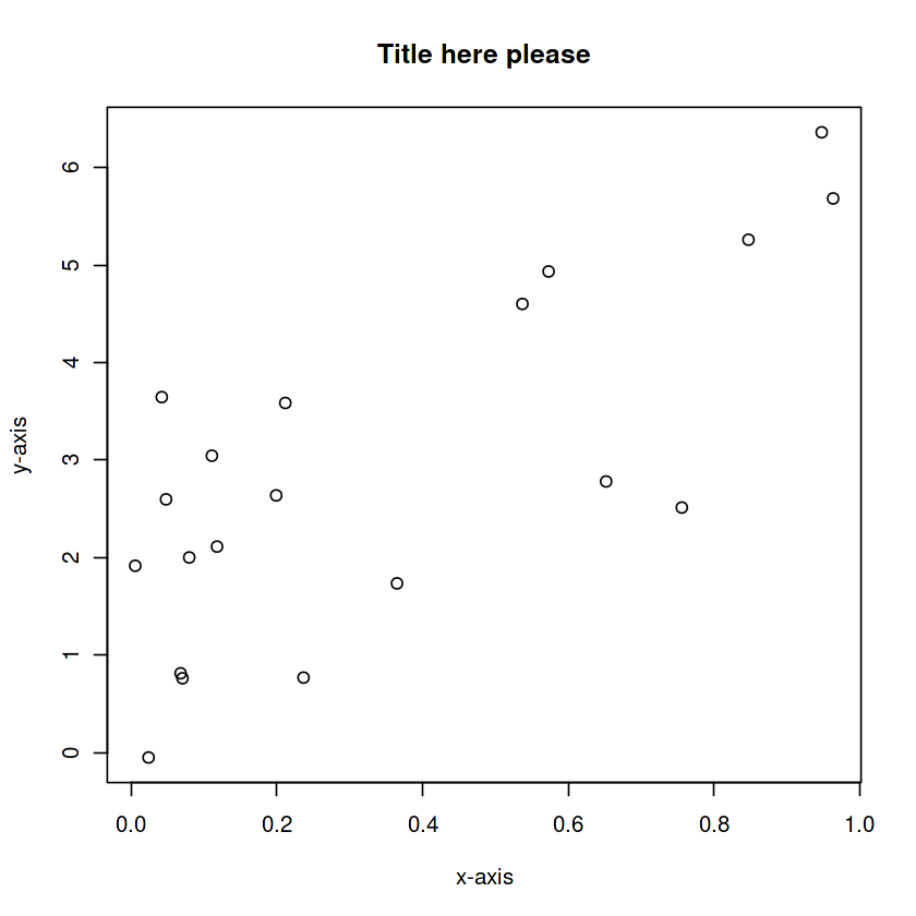
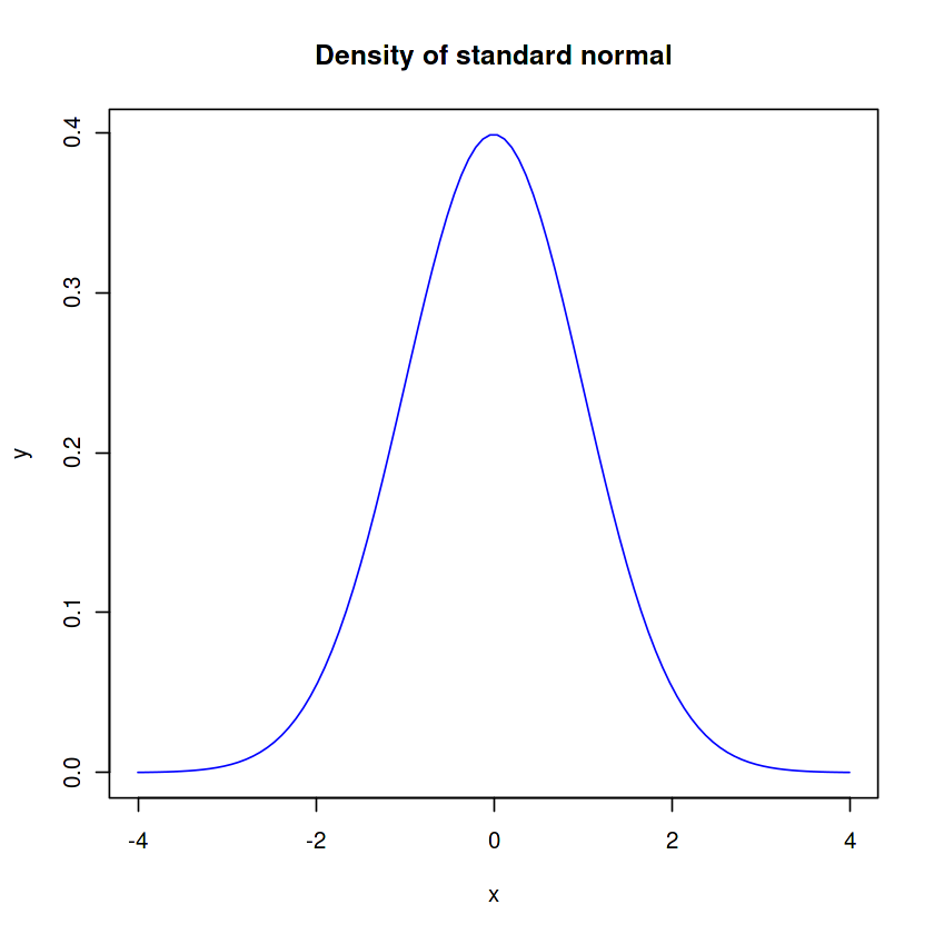
Visualizing data is a very crucial part of any data science project. It helps us convey the message and story the data tells. R has its own library for visualization called ggplot2 which is one of the best visualization libraries out there. We shall cover ggplot2 later in this article, but first, let’s get familiar with the visualization techniques native to the R language.

1. Histogram

age <- titanic$Age  

hist(age, xlab='Age',      
     main="Histogram of passengers Age"
    )

2. Boxplot

y <- rnorm(100, mean=80, sd=3)
boxplot(y, xlab='Y-variable',
       main='boxplot of random variable'
       )

3. Scatterplot

x <- runif(20)
y <- 2 +3*x + rnorm(20)
plot(x, y, 
     xlab='x-axis',
     ylab='y-axis',
     main='Title here please',
    )

4. Line plot

x <- seq(-4, 4, len=100)
y <- dnorm(x, mean=0, sd=1)
plot(x, y, type='l', col='blue')
title('Density of standard normal')

5. Barplot

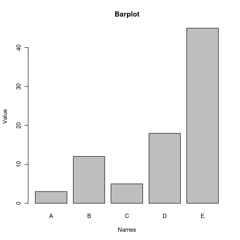
data <- data.frame(
  name=c("A","B","C","D","E") ,  
  value=c(3,12,5,18,45)
) 
barplot(data$value, names.arg=data$name, horiz=FALSE,
       xlab='Names', ylab='Value', main='Barplot')

6. Piechart

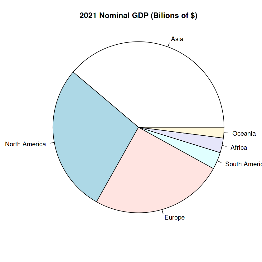
slices <- c(36448.797, 26288.683, 23596.661, 3028.636, 2605.979, 1895.095)
labels <- c("Asia", "North America", "Europe", "South America", "Africa", "Oceania")
pie(slices, labels = labels,
    radius = 2.0,
    main="2021 Nominal GDP (Bilions of $)")

Visualization using ggplot2

The ggplot2 library is built around the ideas introduced in a book called The Grammar of Graphics (Statistics and Computing) It helps us create complex plots with ease using 3 main components: data, coordinate system, and geometry. We can also tell ggplot2 what aesthetics to use like color, shape, size, etc.

syntax:

ggplot(data, aes())+
geom()

data      – dataset used

aes()     – aesthetics

geom() – geometry. here you have a lot of options. I suggest you check out this cheatsheet for a much better grasp of this concept

Let’s get started!

# import ggplot2 library
library(ggplot2)

1. Scatterplot

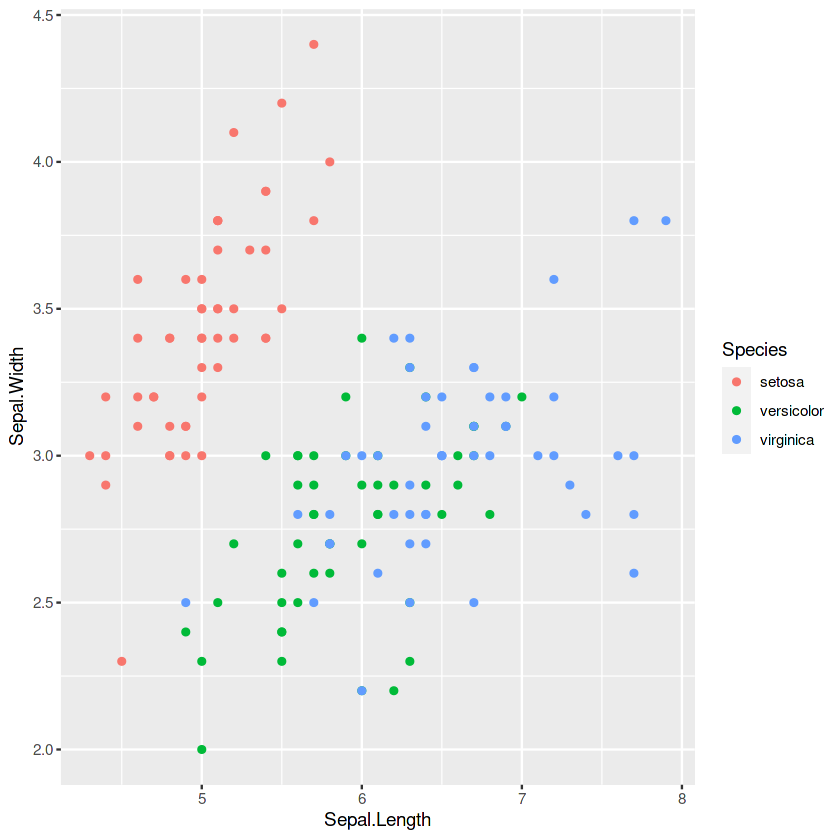
p1 <- ggplot(iris, aes(x = Sepal.Length, y = Sepal.Width, color = Species)) + 
        geom_point()
p1

2. Histogram

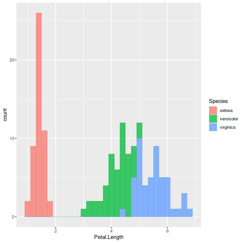
p2 <- ggplot(iris, aes(x = Petal.Length, fill = Species)) +
        geom_histogram(binwidth=0.2, alpha=0.75)
p2

3. Box Plot

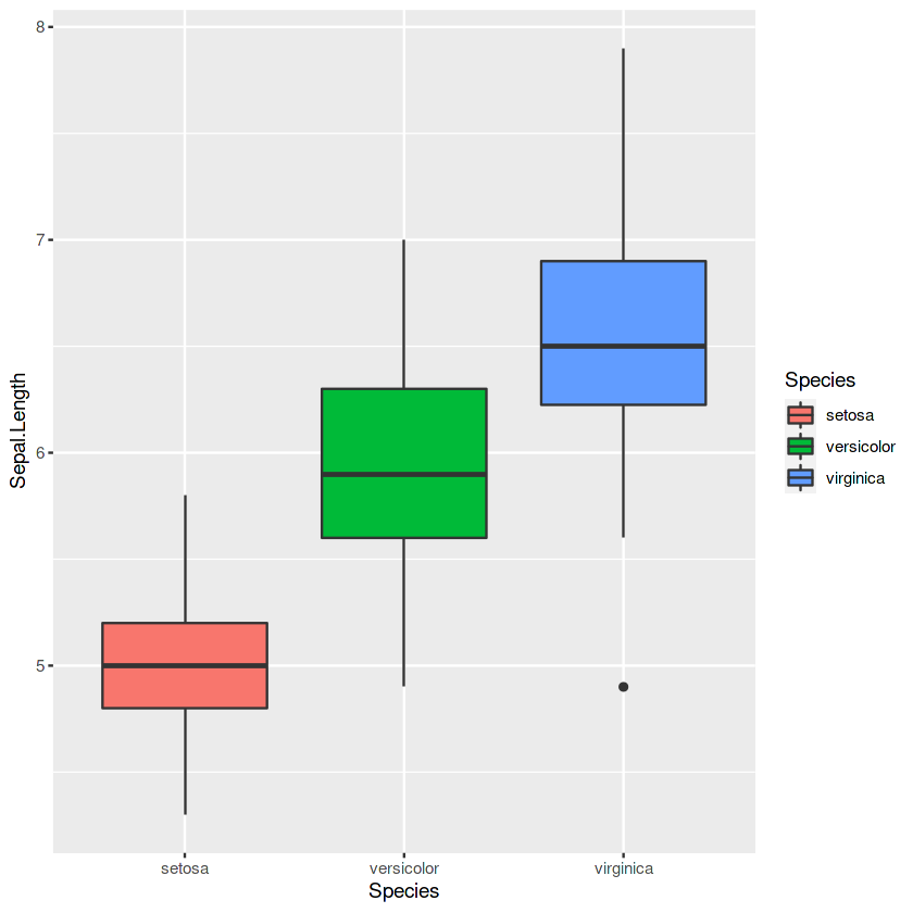
p3 <- ggplot(iris, aes(x = Species, y = Sepal.Length, fill = Species)) +
        geom_boxplot()
p3

4. Barplot

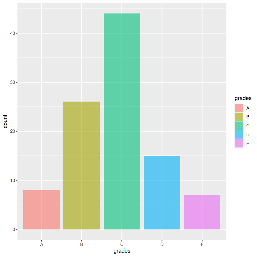
grades <- c('A', 'B', 'C', 'D', 'F')
count <- c(8, 26, 44, 15, 7)

data_grades <- data.frame(x = grades, y = count)

p4 <- ggplot(data_grades, aes(x = grades, y = count, fill = grades)) +
        geom_col(alpha=0.6)
p4

5. Density Plot

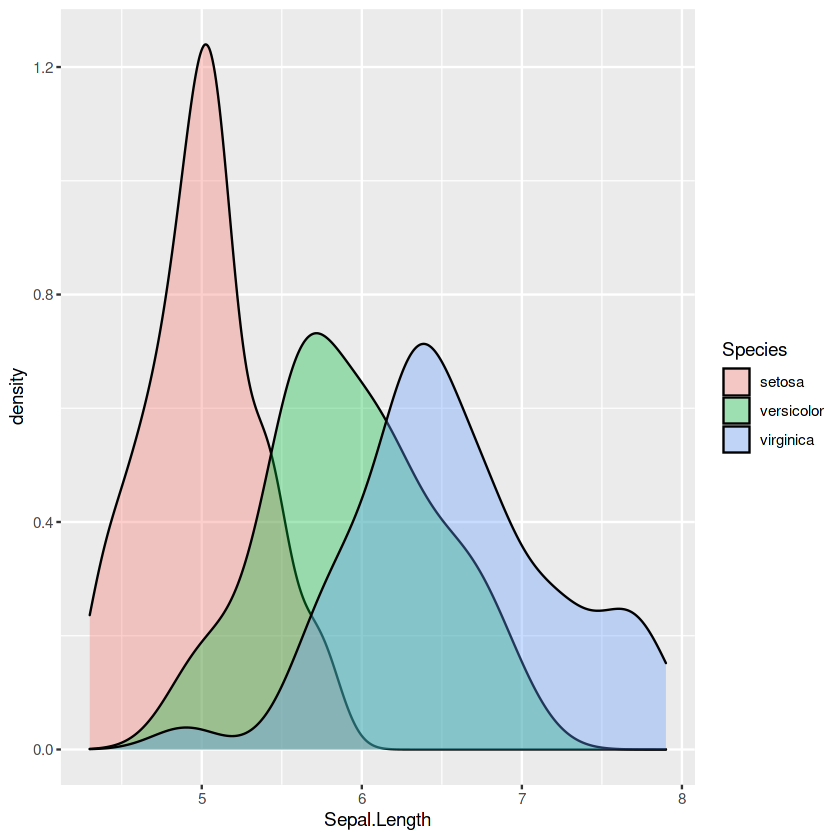
p5 <- ggplot(iris, aes(x = Sepal.Length, fill = Species)) + 
        geom_density(alpha=0.35)
p5

6. Violin Plot

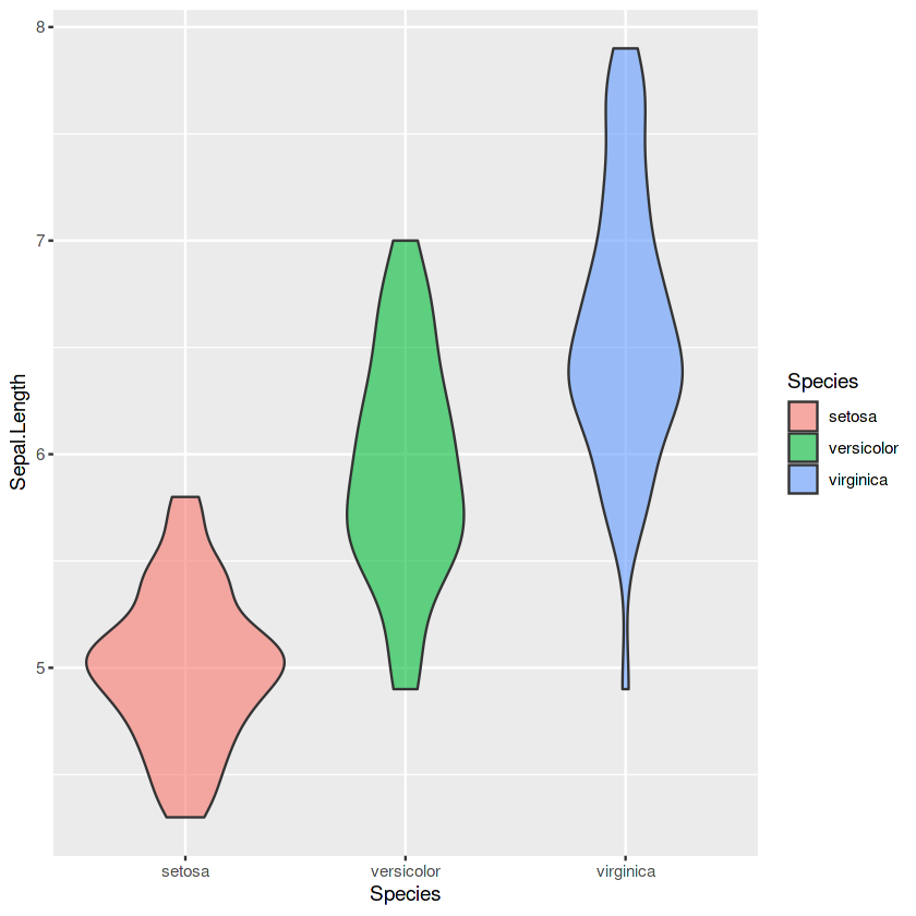
p6 <- ggplot(iris, aes(x = Species, y = Sepal.Length, fill = Species)) +
        geom_violin(alpha=0.6)
p6

7. Pie chart

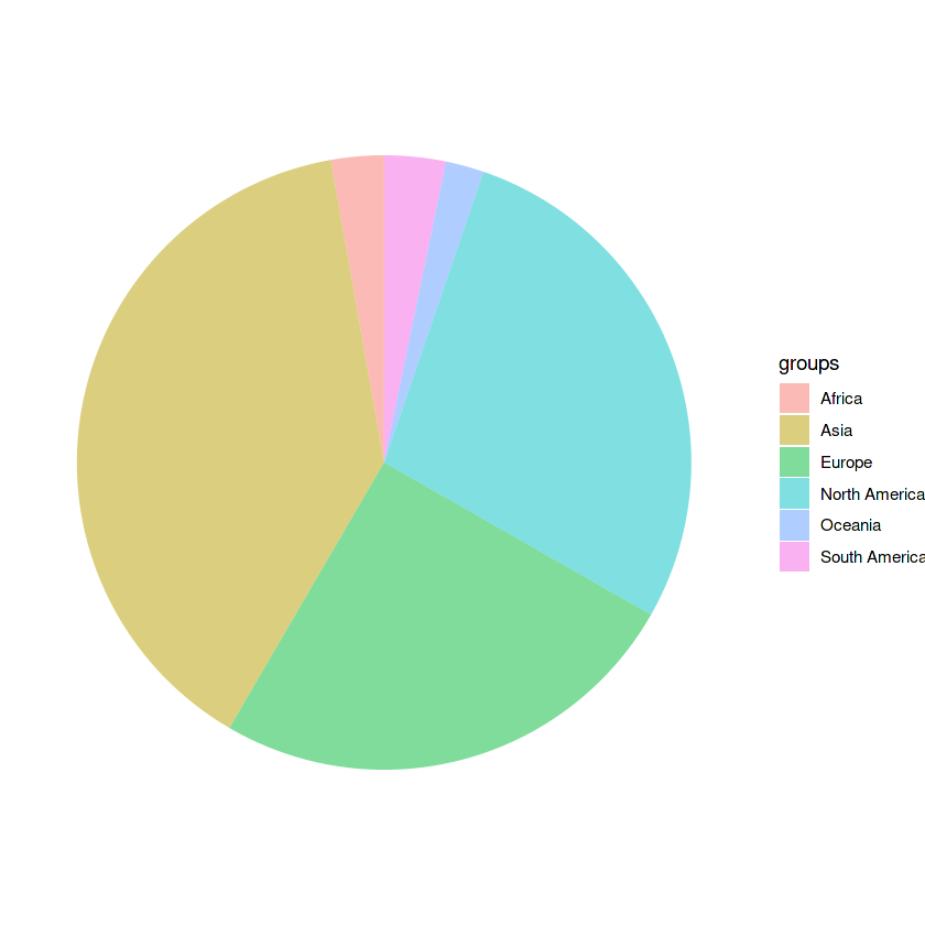
Note: In order to make a pie chart we need to use a combination of geom_bar() and coord_polar()

slices <- c(36448.797, 26288.683, 23596.661, 3028.636, 2605.979, 1895.095)
labels <- c("Asia", "North America", "Europe", "South America", "Africa", "Oceania")

data_gdp <- data.frame(
    values = slices,
    groups = labels
)
ggplot(data_gdp, aes(x="", y=values, fill=groups)) +
  geom_bar(stat="identity", alpha=0.5) +
  coord_polar("y", start=0) + 
  theme_void() # this line is used to clear the background grid

8. Line Plot

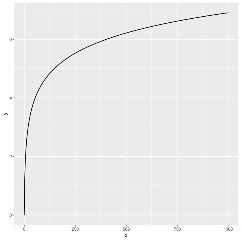
# creating a new dataset
x <- seq(0, 1000, len=500)
y <- log(x + 1)

data <- data.frame(
     x = x, y = y)

# line plot
ggplot(data, aes(x=x, y=y))+
    geom_line()

9. Maps

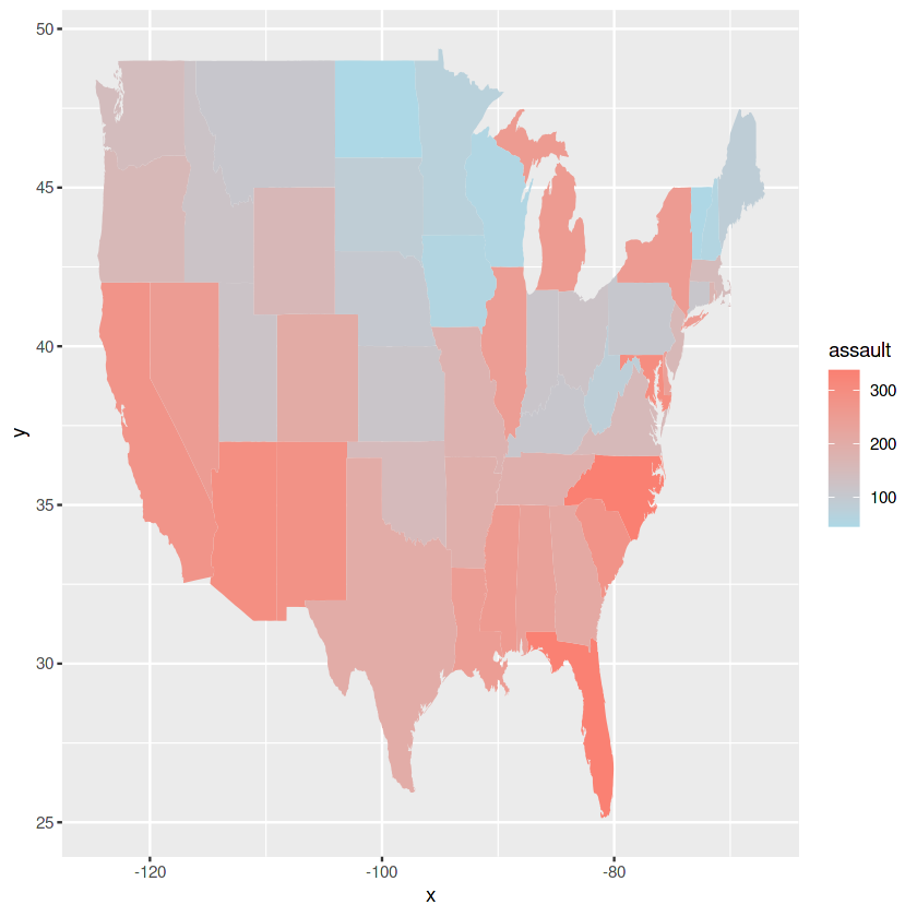
## adaptation of https://www.maths.usyd.edu.au/u/UG/SM/STAT3022/r/current/Misc/data-visualization-2.1.pdf

data <- data.frame(assault = USArrests$Assault, state = tolower(rownames(USArrests)))
map <- map_data("state")

map_plot <- ggplot(data, aes(fill = assault)) + 
                geom_map(aes(map_id = state), map = map,) + 
                expand_limits(x = map$long, y = map$lat)+
                scale_fill_continuous(low = "lightblue", high = "salmon")
map_plot

Correlation Heatmap using corrplot

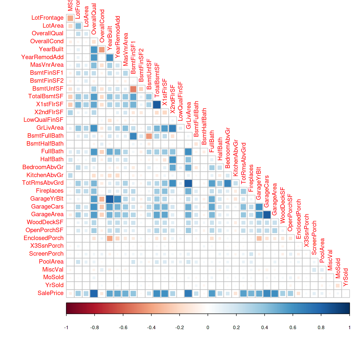
A correlation heatmap is useful to plot the correlation between multiple variables. In this example, we will use the library corrplot to create a correlation heatmap on the House Price dataset.

#importing library
library(corrplot)

options(repr.plot.width = 10, repr.plot.height = 10)

numeric_var <- names(house)[which(sapply(house, is.numeric))]
house_cont <- house[numeric_var]

correlations <- cor(na.omit(house_cont[,-1]))
corrplot(correlations, method="square", type='lower', diag=FALSE)

Endnotes

In this article, we started with the basics and saw what are variables and how to assign values to them. Next, we got familiar with the native data types and common data structures used in R. Then we learned how to extract desired parts from these data structures. Then, at last, we learned how to import data and how to use different control structures like loops and conditional statements in R.

Then we got familiar with the data analysis part of using R. We learned how to create customs functions and then started with manipulating data frames using dplyr. Next, we dived into visualizations using both native R and a robust viz library called gglot2. Thank you for reading my article. I hope you liked it.

You can read my other articles at:

Sion | Author at Analytics Vidhya

References

Image 1 : https://www.r-project.org/logo/

Sion 14 Sep, 2021