This article was published as a part of the Data Science Blogathon

Optuna is an automatic hyperparameter tuning software framework, particularly designed for Machine Learning, and can use it with other frameworks like PyTorch, TensorFlow, Keras, SKlearn, etc.
Optuna uses something called define-by-run API which helps the user to write high modular code and dynamically construct the search spaces for the hyperparameters, which we’ll learn later in this article. Different samplers like grid search, Random, Bayesian and Evolutionary algorithms are used to automatically find the optimal parameter. Let’s have a brief discussion about the different samplers available in Optuna.
But what makes it so popular among Kagglers? Here are the key features which they’ve mentioned on the website:
1) Lightweight and versatile: A simple installation is needed and then you are ready to go. Can handle a wide range of tasks and find the best-tuned alternative.
2) Eager Search Spaces: Familiar Pythonic syntaxes like conditionals and loops are used to automatically search for optimal hyperparameters.
3) State-of-the-art Algorithms: Quickly searches large spaces and prunes unpromising trials faster for better and quick results.
4) Easy Parallelization: Can easily parallelize hyperparameter searches with little or no changes to the original code.
5) Quick visualizations: Various visualization features are also available to analyze optimization results visually.
Before beginning with the tutorial, we have to understand a few Optuna terminologies and conventions:
In Optuna, there are two major terminologies, namely:
1) Study: The whole optimization process is based on an objective function i.e the study needs a function which it can optimize.
2) Trial: A single execution of the optimization function is called a trial. Thus the study is a collection of trials.
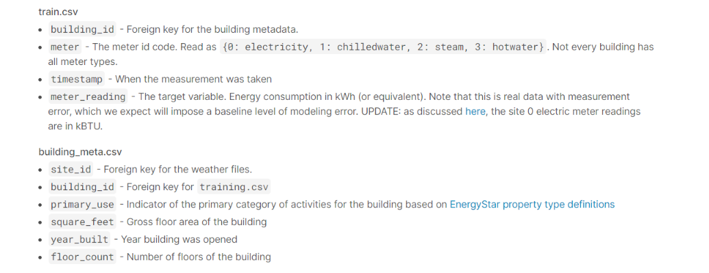
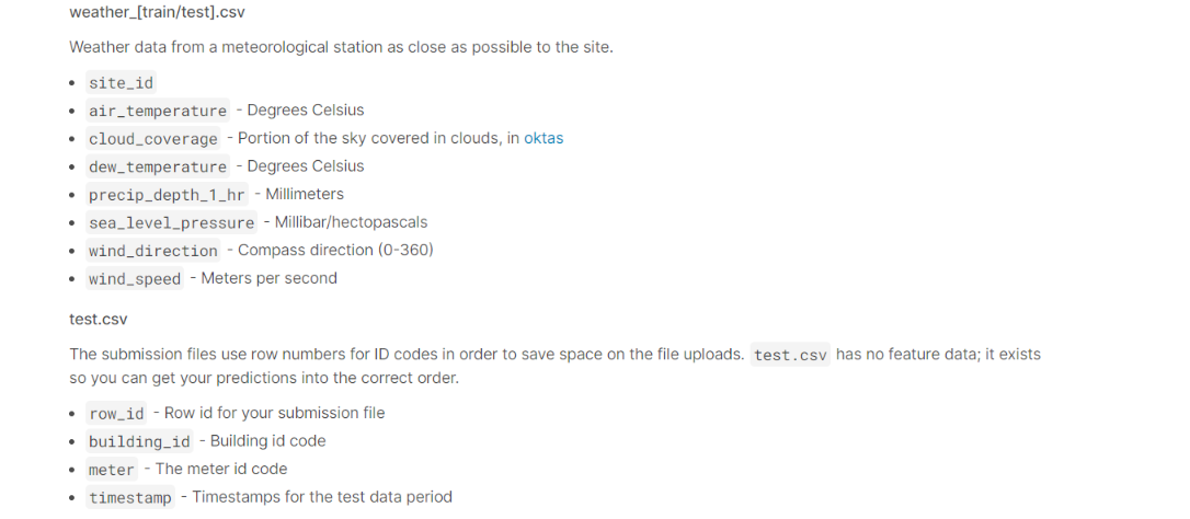
For this article, we will use the dataset from ASHRAE – Great Energy Predictor III which is a Kaggle competition to predict the amount of energy consumed by a building. The dataset has a size of 2.5 Gb, so it’s quite heavy.
The data is divided into few files for ease of use. To train our model we are provided with train.csv, weather_train.csv, and building_metadata.csv. along with that, we have a few trs.csv files too. Here is a brief description of the files, along with the columns present.
import gc
import os
from pathlib import Path
import random
import sys

from tqdm import tqdm_notebook as tqdm
import numpy as np # linear algebra
import pandas as pd # data processing

import matplotlib.pyplot as plt
import seaborn as sns

from IPython.core.display import display, HTML

# --- plotly ---
from plotly import tools, subplots
import plotly.offline as py
py.init_notebook_mode(connected=True)
import plotly.graph_objs as go
import plotly.express as px
import plotly.figure_factory as ff

# --- models ---
from sklearn import preprocessing
from sklearn.model_selection import KFold
import lightgbm as lgb
import xgboost as xgb
import catboost as cb%%time
# Read data...
root = '../input/ashrae-energy-prediction'
train_df = pd.read_csv(os.path.join(root, 'train.csv'))
weather_train_df = pd.read_csv(os.path.join(root, 'weather_train.csv'))
test_df = pd.read_csv(os.path.join(root, 'test.csv'))
weather_test_df = pd.read_csv(os.path.join(root, 'weather_test.csv'))
building_meta_df = pd.read_csv(os.path.join(root, 'building_metadata.csv'))
sample_submission = pd.read_csv(os.path.join(root, 'sample_submission.csv'))
Our aim for this competition will be to predict the energy consumption of buildings. The 4 types of energy we have to predict are:
|
|
|
|
|
|
|
|
|
|
Electricity and water consumption might vary and have different predicting factors. So I’ve separately trained and predicted the models.
train_df['date'] = train_df['timestamp'].dt.date
train_df['meter_reading_log1p'] = np.log1p(train_df['meter_reading'])
def plot_date_usage(train_df, meter=0, building_id=0):
train_temp_df = train_df[train_df['meter'] == meter]
train_temp_df = train_temp_df[train_temp_df['building_id'] == building_id]
train_temp_df_meter = train_temp_df.groupby('date')['meter_reading_log1p'].sum()
train_temp_df_meter = train_temp_df_meter.to_frame().reset_index()
fig = px.line(train_temp_df_meter, x='date', y='meter_reading_log1p')
fig.show()plot_date_usage(train_df, meter=0, building_id=0)
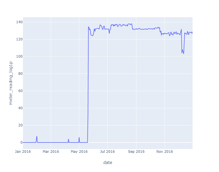
As you can see, the data before mid-May 2016 looks weird, since it’s at the bottom of the graph. The reason for this is that all the electricity meter readings are 0 until May 20 for site_id == 0. This was pointed out by a participant. Thus the logical thing to do is get rid of that segment of the data.
building_meta_df[building_meta_df.site_id == 0]
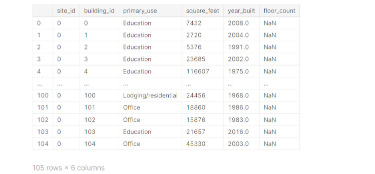
Thus we can see that all the entries with site_id == 0 have building_id <= 104. Now we get rid of them:
train_df = train_df.query('not (building_id <= 104 & meter == 0 & timestamp <= "2016-05-20")')
We can use the timestamp feature for better features.
def preprocess(df):
    df["hour"] = df["timestamp"].dt.hour
    df["month"] = df["timestamp"].dt.month
    df["dayofweek"] = df["timestamp"].dt.dayofweek
    df["weekend"] = df["dayofweek"] >= 5
preprocess(train_df)
df_group = train_df.groupby(['building_id', 'meter'])['meter_reading_log1p']
building_mean = df_group.mean().astype(np.float16)
building_median = df_group.median().astype(np.float16)
building_min = df_group.min().astype(np.float16)
building_max = df_group.max().astype(np.float16)
building_std = df_group.std().astype(np.float16)
building_stats_df = pd.concat([building_mean, building_median, building_min, building_max, building_std], axis=1,
                              keys=['building_mean', 'building_median', 'building_min', 'building_max', 'building_std']).reset_index()
train_df = pd.merge(train_df, building_stats_df, on=['building_id', 'meter'], how='left', copy=False)
train_df.head()

(Note: All the columns are not included in the above snippet)
The weather data has a lot of NaN values, so we can’t just get rid of the entries. We’ll try to fill these values by interpolating data.
weather_train_df.head()
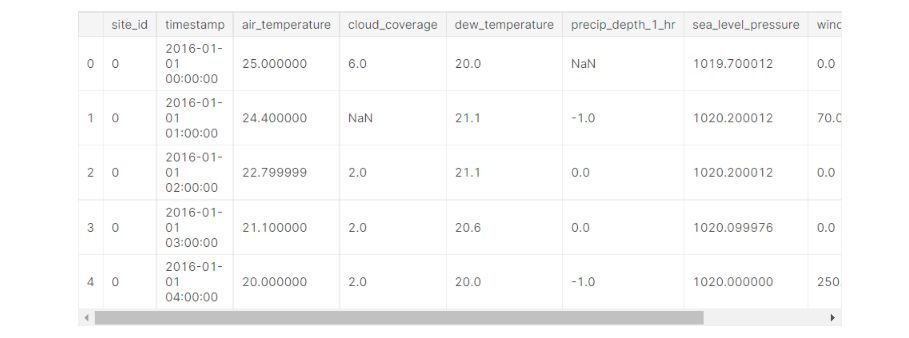
weather_train_df.isna().sum()

weather_test_df = pd.read_feather(root/'weather_test.feather')
weather = pd.concat([weather_train_df, weather_test_df],ignore_index=True)
del weather_test_df
weather_key = ['site_id', 'timestamp']
temp_skeleton = weather[weather_key + ['air_temperature']].drop_duplicates(subset=weather_key).sort_values(by=weather_key).copy()
temp_skeleton['temp_rank'] = temp_skeleton.groupby(['site_id', temp_skeleton.timestamp.dt.date])['air_temperature'].rank('average')
df_2d = temp_skeleton.groupby(['site_id', temp_skeleton.timestamp.dt.hour])['temp_rank'].mean().unstack(level=1)
site_ids_offsets = pd.Series(df_2d.values.argmax(axis=1) - 14)
site_ids_offsets.index.name = 'site_id'
def timestamp_align(df):
df['offset'] = df.site_id.map(site_ids_offsets)
df['timestamp_aligned'] = (df.timestamp - pd.to_timedelta(df.offset, unit='H'))
df['timestamp'] = df['timestamp_aligned']
del df['timestamp_aligned']
return df
del weather
del temp_skeleton
gc.collect()weather_train_df = timestamp_align(weather_train_df)
weather_train_df = weather_train_df.groupby('site_id').apply(lambda group: group.interpolate(limit_direction='both'))
Now the number of NaN values has decreased significantly in our dataset.
def add_lag_feature(weather_df, window=3):
    group_df = weather_df.groupby('site_id')
    c = ['dew_temperature', 'cloud_coverage', 'precip_depth_1_hr', 'air_temperature', 'sea_level_pressure', 'wind_direction', 'wind_speed']
    cols = c
    rolled = group_df[cols].rolling(window=window, min_periods=0)
    lag_mean = rolled.mean().reset_index().astype(np.float16)
    lag_max = rolled.max().reset_index().astype(np.float16)
    lag_min = rolled.min().reset_index().astype(np.float16)
    lag_std = rolled.std().reset_index().astype(np.float16)
    for col in cols:
        weather_df[f'{col}_mean_lag{window}'] = lag_mean[col]
        weather_df[f'{col}_max_lag{window}'] = lag_max[col]
        weather_df[f'{col}_min_lag{window}'] = lag_min[col]
        weather_df[f'{col}_std_lag{window}'] = lag_std[col]
add_lag_feature(weather_train_df, window=3) add_lag_feature(weather_train_df, window=72)
Now that lags are added, we’ll categorize the primary_use column to reduce the memory on merge:
primary_use_list = building_meta_df['primary_use'].unique()
primary_use_dict = {key: value for value, key in enumerate(primary_use_list)}
print('primary_use_dict: ', primary_use_dict)
building_meta_df['primary_use'] = building_meta_df['primary_use'].map(primary_use_dict)

gc.collect()

In this section, we will learn how to work with Optuna. But first, let’s divide our columns into categorical values and numeric features.
category_columns = ['building_id', 'site_id', 'primary_use']
weather_columns = [
    'air_temperature', 'cloud_coverage',
    'dew_temperature', 'precip_depth_1_hr', 'sea_level_pressure',
    'wind_direction', 'wind_speed', 'air_temperature_mean_lag72',
    'air_temperature_max_lag72', 'air_temperature_min_lag72',
    'air_temperature_std_lag72', 'cloud_coverage_mean_lag72',
    'dew_temperature_mean_lag72', 'precip_depth_1_hr_mean_lag72',
    'sea_level_pressure_mean_lag72', 'wind_direction_mean_lag72',
    'wind_speed_mean_lag72', 'air_temperature_mean_lag3',
    'air_temperature_max_lag3',
    'air_temperature_min_lag3', 'cloud_coverage_mean_lag3',
    'dew_temperature_mean_lag3',
    'precip_depth_1_hr_mean_lag3', 'sea_level_pressure_mean_lag3',
    'wind_direction_mean_lag3', 'wind_speed_mean_lag3']
feature_columns = ['square_feet', 'year_built'] + [
    'hour', 'weekend', 'dayofweek', # 'month'
    'building_median'] + weather_cols
def create_X_y(train_df, target_meter):
target_train_df = train_df[train_df['meter'] == target_meter]
target_train_df = target_train_df.merge(building_meta_df, on='building_id', how='left')
target_train_df = target_train_df.merge(weather_train_df, on=['site_id', 'timestamp'], how='left')
X_train = target_train_df[feature_cols + category_cols]
y_train = target_train_df['meter_reading_log1p'].values
del target_train_df
return X_train, y_train
Every hyperparameter tuning project done with Optuna begins with an objective function where we have to decide the metrics on which we base our optimization. A trial object is the input in an objective method and returns a score.
def objective(trial, ...):
    # calculate score...
    return score
Now we’ll train a LightGBM model for the electricity meter, get the best validation score and return this score as the final score. Let’s begin!!
import optuna
from optuna import Trial
debug = False
train_df_original = train_df
# Only using 10000 data,,, for fast computation for debugging.
train_df = train_df.sample(10000)def objective(trial: Trial, fast_check=True, target_meter=0, return_info=False):
folds = 5
seed = 666
shuffle = False
kf = KFold(n_splits=folds, shuffle=shuffle, random_state=seed)
X_train, y_train = create_X_y(train_df, target_meter=target_meter)
y_valid_pred_total = np.zeros(X_train.shape[0])
gc.collect()
print('target_meter', target_meter, X_train.shape)
L = [X_train.columns.get_loc(cat_col) for cat_col in category_cols]
categorical_features = L
print('cat_features', categorical_features)
models = []
valid_score = 0
for train_idx, valid_idx in kf.split(X_train, y_train):
train_data = X_train.iloc[train_idx,:], y_train[train_idx]
valid_data = X_train.iloc[valid_idx,:], y_train[valid_idx]
print('train', len(train_idx), 'valid', len(valid_idx))
a, b, c = fit_lgbm(trial, train_data, valid_data, cat_features=category_cols,
num_rounds=1000)
model, y_pred_valid, log = a, b, c
y_valid_pred_total[valid_idx] = y_pred_valid
models.append(model)
gc.collect()
valid_score += log["valid/l2"]
if fast_check:
break
valid_score /= len(models)
if return_info:
return valid_score, models, y_pred_valid, y_train
else:
return valid_scoreThe fit_lgbm function has the core training code and defines the hyperparameters.
Next, we’ll get familiar with the inner workings of the “trial” module next.
Here is a comparison between using Optuna vs conventional Define-and-run code:
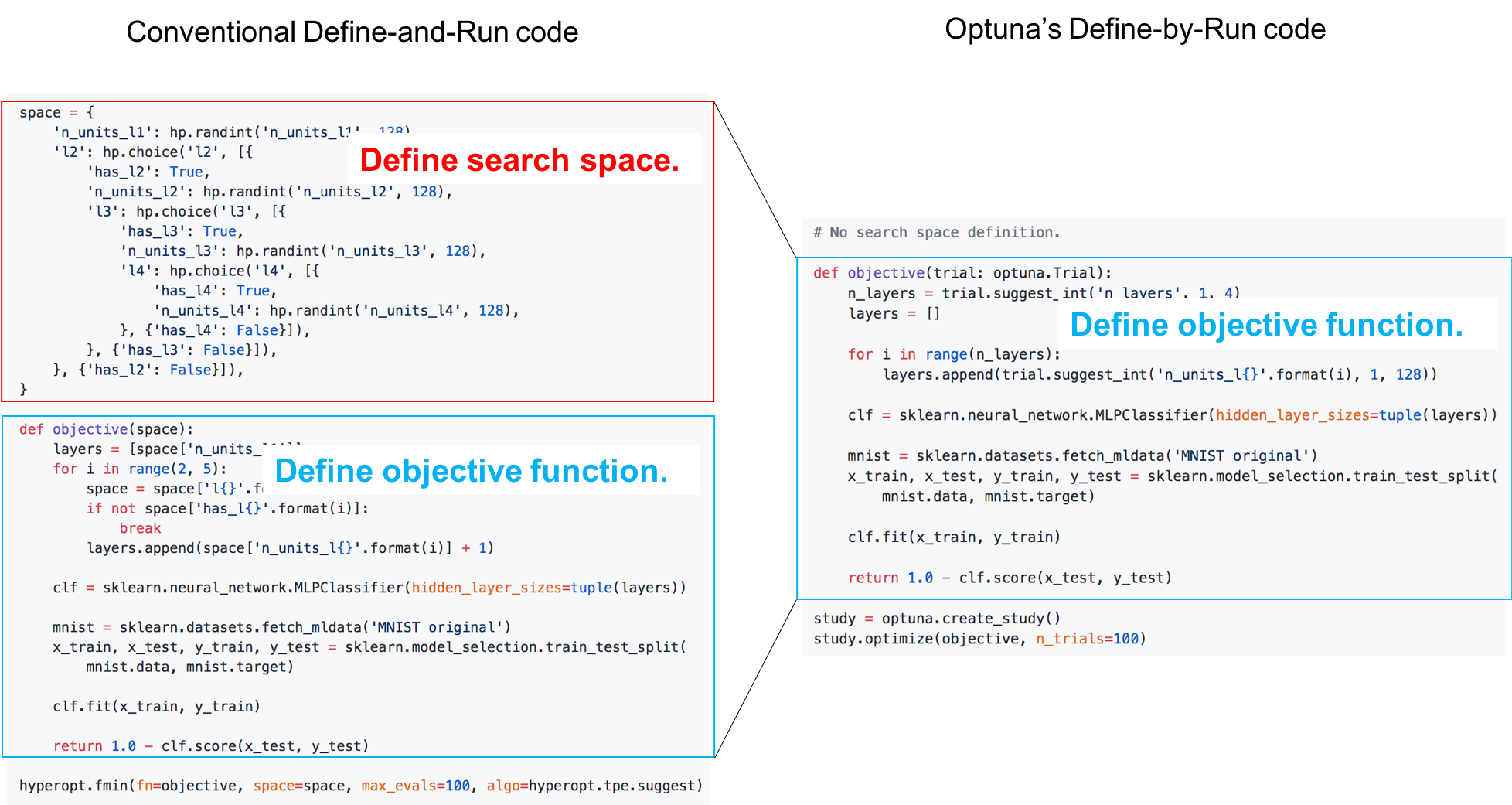
This is the advantage of Define-by-run. which makes it easier for the user to write intuitive code to get the hyperparameters, instead of defining the whole search space in advance.
You can use these methods to get the hyperparameters:
# Categorical parameter
optimizer = trial.suggest_categorical('optimizer', ['MomentumSGD', 'Adam'])

# Int parameter
num_layers = trial.suggest_int('num_layers', 1, 3)

# Uniform parameter
dropout_rate = trial.suggest_uniform('dropout_rate', 0.0, 1.0)

# Loguniform parameter
learning_rate = trial.suggest_loguniform('learning_rate', 1e-5, 1e-2)

# Discrete-uniform parameter
drop_path_rate = trial.suggest_discrete_uniform('drop_path_rate', 0.0, 1.0, 0.1)
Now let’s create a simple Lightgbm model:
def fit_lgbm(trial, train, val, devices=(-1,), seed=None, cat_features=None, num_rounds=1500):
    """Train Light GBM model"""
    X_train, y_train = train
    X_valid, y_valid = val
    metric = 'l2'
    params = {
        'num_leaves': trial.suggest_int('num_leaves', 2, 256),
        'objective': 'regression',
        'max_depth': -1,
        'learning_rate': 0.1,
        "boosting": "gbdt",
        'lambda_l1': trial.suggest_loguniform('lambda_l1', 1e-8, 10.0),
        'lambda_l2': trial.suggest_loguniform('lambda_l2', 1e-8, 10.0),
        "bagging_freq": 5,
        "bagging_fraction": trial.suggest_uniform('bagging_fraction', 0.1, 1.0),
        "feature_fraction": trial.suggest_uniform('feature_fraction', 0.4, 1.0),
        "metric": metric,
        "verbosity": -1,
    }
    device = devices[0]
    if device == -1:
        # use cpu
        pass
    else:
        # use gpu
        print(f'using gpu device_id {device}...')
        params.update({'device': 'gpu', 'gpu_device_id': device})

    params['seed'] = seed

    early_stop = 20
    verbose_eval = 20

    d_train = lgb.Dataset(X_train, label=y_train, categorical_feature=cat_features)
    d_valid = lgb.Dataset(X_valid, label=y_valid, categorical_feature=cat_features)
    watchlist = [d_train, d_valid]

    print('training LGB:')
    model = lgb.train(params,
                      train_set=d_train,
                      num_boost_round=num_rounds,
                      valid_sets=watchlist,
                      verbose_eval=verbose_eval,
                      early_stopping_rounds=early_stop)

    # predictions
    y_pred_valid = model.predict(X_valid, num_iteration=model.best_iteration)

    print('best_score', model.best_score)
    log = {'train/l2': model.best_score['training']['l2'],
           'valid/l2': model.best_score['valid_1']['l2']}
    return model, y_pred_valid, log
Now Time for Optimization!
After defining an objective function and finding hyperparameters using the ‘trial‘ module, we are all set for our tuning. Just 2 lines of code and all the hyperparameter tuning will be done for you!!
study = optuna.create_study()
study.optimize(objective, n_trials=10)
Since the value of n_trials is 10, the output is quite large. Thus in the below screenshot, I’ll include just the last trial:
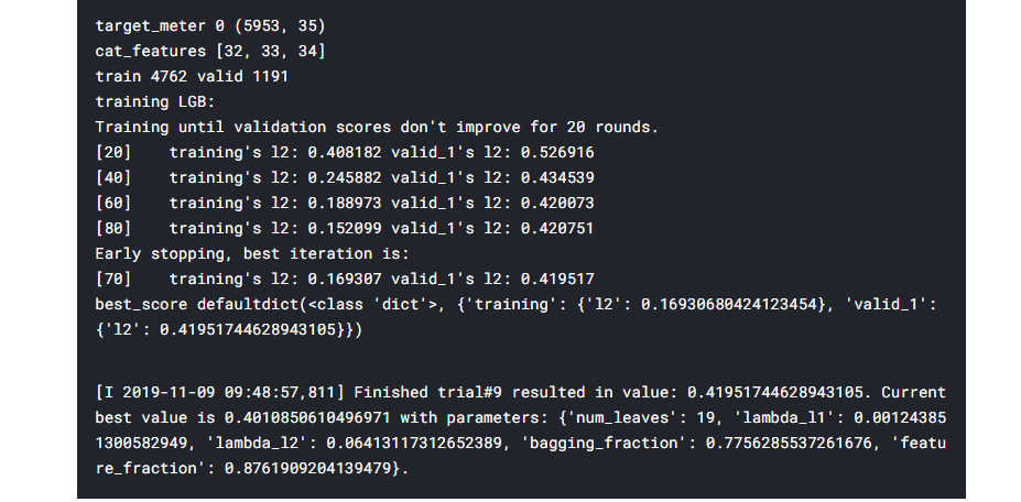
And that’s it!! your Hyperparameters are tuned!!
Trial manages all the single execution of model training, evaluation, and getting score by specifying one trial of the hyperparameter.
Study manages and records all the entirety of Trials executed. This record helps us to know the best hyperparameter and suggests the next parameter space to search.
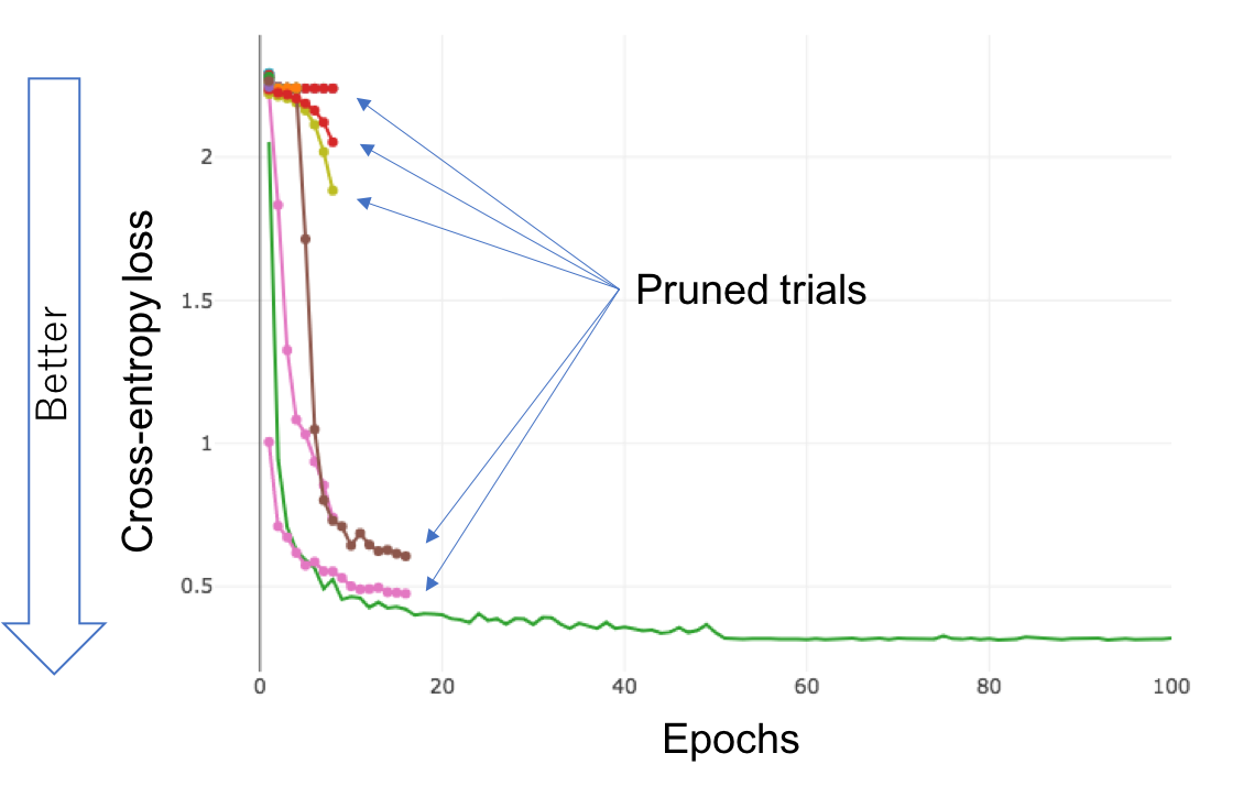
One of the advanced and useful techniques in optuna is Pruning of the unpromising trials. For those who are unfamiliar with what pruning is, it is a technique to compress data in ML search algorithms that reduces the size of a decision tree by eliminating redundant and unimportant data to classify instances.
Thus pruning can improve upon the complexity of the final classifier and combat overfitting. Integration for multiple popular ML frameworks is provided in Optuna using which the user can try pruning during hyperparameter training. Examples:
optuna.integration.XGBoostPruningCallbackoptuna.integration.LightGBMPruningCallbackoptuna.integration.ChainerPruningExtensionoptuna.integration.KerasPruningCallbackoptuna.integration.TensorFlowPruningHookoptuna.integration.TFKerasPruningCallbackoptuna.integration.MXNetPruningCallbackYou can read in detail about these integrations here: optuna.integration.
Here’s a simple example of creating an objective function with pruning:
def objective_with_prune(trial: Trial, fast_check=True, target_meter=0):
    folds = 5
    seed = 666
    shuffle = False
    kf = KFold(n_splits=folds, shuffle=shuffle, random_state=seed)

    X_train, y_train = create_X_y(train_df, target_meter=target_meter)
    y_valid_pred_total = np.zeros(X_train.shape[0])
    gc.collect()
    print('target_meter', target_meter, X_train.shape)
    x = [X_train.columns.get_loc(cat_col) for cat_col in category_cols]
    cat_features = x
    print('cat_features', cat_features)

    models0 = []
    valid_score = 0
    for train_idx, valid_idx in kf.split(X_train, y_train):
        train_data = X_train.iloc[train_idx,:], y_train[train_idx]
        valid_data = X_train.iloc[valid_idx,:], y_train[valid_idx]

        print('train', len(train_idx), 'valid', len(valid_idx))
        model, y_pred_valid, log = fit_lgbm_with_pruning(trial, train_data, valid_data, cat_features=category_cols,
                                                         num_rounds=1000)
        y_valid_pred_total[valid_idx] = y_pred_valid
        models0.append(model)
        gc.collect()
        valid_score += log["valid/l2"]
        if fast_check:
            break
    valid_score /= len(models0)
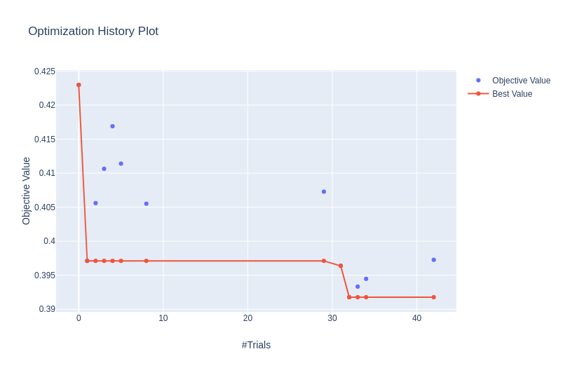
return valid_scoreOptuna provides us with the option to visualize the training and study history to determine the hyperparameter with the best performance. And the best thing, all these visualizations just need 1 line of code!!!
optuna.visualization.plot_optimization_history(study)
optuna.visualization.plot_intermediate_values(study)
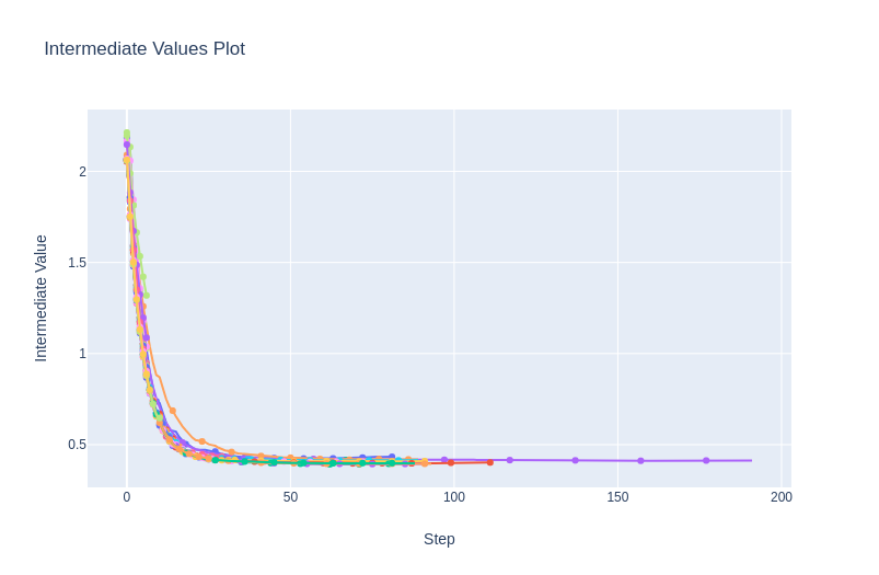
All the different colours show the loss curve of each trial.
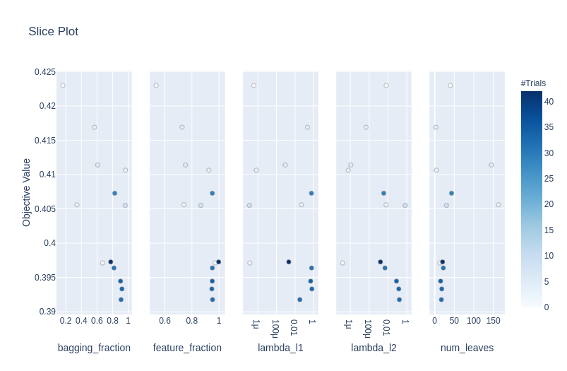
optuna.visualization.plot_slice(study)
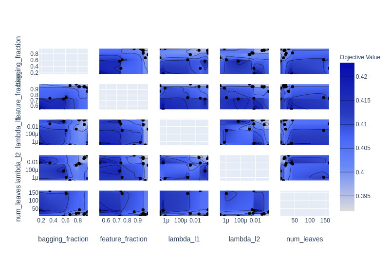
Plotting a parameter pair with the objective value as a contour.
optuna.visualization.plot_contour(study)
optuna.visualization.plot_parallel_coordinate(study)
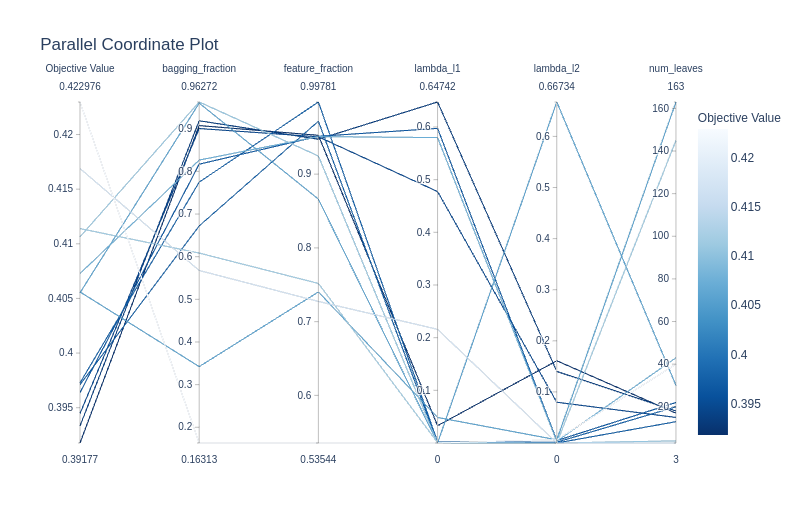
This article was just the beginning of getting familiar with Optuna and covered most of the basics as to how to tune the hyperparameters of your ML model. We learned the terminologies used in the Optuna library like trials and study. We also learned how to define an objective function which is mandatory for using the Optuna tuning.
Next, we discussed and worked on some advanced concepts like Pruning, which is also one of the best features of Optuna. Then we learned how to use the visualizations of Optuna and use them to evaluate and select the best Hyperparameters.
Here’s a video I suggest you should watch:
Thanks for reading my article, I hope you enjoyed reading it as much as I enjoyed writing it. Cheers!!!
References
Dataset – https://www.kaggle.com/c/ashrae-energy-prediction/overview
Image 1 – https://optuna.org/
Image 2 – https://optuna.org/
Optuna is better than grid search because it’s brighter. It learns from past tries, uses resources wisely, and can handle different choices. Optuna is faster and more flexible than grid search, making it a better choice for finding the best settings for machine learning
Optuna simplifies and automates the hyperparameter tuning process, saving time and resources while improving model accuracy.
Optuna is versatile and can be applied to various machine-learning tasks, making it a popular choice across different domains.
Lorem ipsum dolor sit amet, consectetur adipiscing elit,