This article was published as a part of the Data Science Blogathon
Welcome to the second regression tutorial – level intermediate. If you haven’t read the tutorial AutoML using Pycaret with a Regression Use-Case, I strongly recommend you to read the first one to understand the basics of working in PyCaret:
In this article, we will use the pycaret.regression module to learn :
Normalization: normalizing and scaling the dataset.
Transformation: applying transformations that make the data linear and approximately normal.
Target Transformation: applying transformations to the target variable.
Combine Rare levels: combining rare levels in categorical features.
Bin numeric variables: binning numeric variables and transforming numeric features into categorical ones using the ‘sturges’ rule
Model Ensembling and Stacking: boosting model performance with multiple ensembling techniques like Bagging, Boosting, Voting, and Generalized Stacking.
Experiment Logging: logging experiments in PyCaret using MLFlow backend.
Python 3.6 or higher
PyCaret 2.0 or higher
Stable internet connection to load the data
Completion of AutoML using Pycaret: Regression – Beginner
Before we dive into the practical use of the techniques mentioned above, it is important to brush up on the topics briefly and when to use them. Mostly these techniques help with linear and parametric algorithms, however significant performance gains can also be seen on tree-based models. The descriptions included here are quite brief and I recommend you to read some other reference materials if this is not sufficient for you.
Often used interchangeably with Scaling or standardization, is used to transform the actual numeric values in such a way that provides helpful properties for machine learning. Algorithms like Linear Regression, Support Vector Machine, and K Nearest Neighbours assume that the features are centred around Zero and have variances that are in the same level of order. If some feature has a variance that is larger in order of magnitude than other features, the model might not understand all features correctly and could perform poorly.
Normalization scales the range of the data to remove the impact of magnitude in the variance, whereas transformation is a much more radical technique to change the shape of the distribution so that the transformed data can be represented by a normal or an approximately normal distribution. Generally one should transform the data if using algorithms that assume normality or Gaussian distribution. Some examples of these algorithms are Linear Regression, Lasso Regression, and Ridge Regression.
It’s similar to the transformation technique explained above with the exception that this is only applied to the target variable. You can read more here to understand the effects of target transformation.
Many a time categorical features have levels that are insignificant in the frequency distribution. These levels might introduce noise into the dataset due to the limited sample size of learning. One way of dealing with these rare levels is to combine them in a new class.
Binning is the process of transforming numeric variables into categorical features. Binning sometimes improves the accuracy of the predictive model by reducing the noise or non-linearity in the data. Sturges rule is used by PyCaret to automatically determine the number and size of the bins.
Ensembling is a technique where multiple diverse models are created to predict an outcome. Either different modeling algorithms are used or different samples of training data set. These ensemble models are used to reduce the generalization error of the prediction. The two most common ensembling methods are Bagging and Boosting. Stacking is also a type of ensemble learning where the outputs from numerous models are used as inputs for a meta-model to predict the outcome. You can read more about ensembling here.
We shall learn how to do hyperparameter tuning for an ensemble model which is similar to the tuning of a simple ML model.

In this article, we will use the dataset called “Sarah Gets a Diamond”. The story is about an MBA student choosing the right diamond for his future wife, Sarah. The dataset contains 6000 entries for training and has 9 columns named:
You can easily load the data from PyCaret’s data repository if you have a stable internet connection:
from pycaret.datasets import get_data
dataset = get_data('diamond', profile=True)
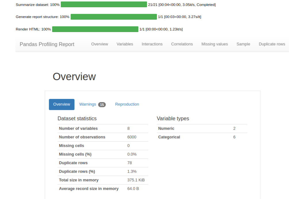
Since the profile parameter is set to True, an interactive data profile with an overview of the data and Exploratory data analysis of the data is received. This is a very comprehensive analysis, I’ve included a screenshot of a small part below.
#check the shape of data
dataset.shape
> (6000,8)
A sample of 600 has been withheld from the original dataset to demonstrate the predict_model() function on unseen data. Caution: These unseen entries should not be confused with train/test split. These 600 records can be seen as not available at the time of the ML experiment.
data = dataset.sample(frac=0.9, random_state=786)
data_unseen = dataset.drop(data.index)
data.reset_index(drop=True, inplace=True)
data_unseen.reset_index(drop=True, inplace=True)
print('Data for Modeling: ' + str(data.shape))
print('Unseen Data For Predictions ' + str(data_unseen.shape))
> Data for Modeling: (5400, 8)
> Unseen Data For Predictions (600, 8)
In our previous article, we learned how to use setup() to initialize the environment in PyCaret. We use just a few additional parameters in our previous article as we did not perform any preprocessing steps. In this article, I’ll show you how to take it to the next level by customizing the preprocessing pipeline using setup().
exp_reg102 = setup(data = data, target = 'Price', session_id=123,
                  normalize = True, transformation = True, transform_target = True,
                  combine_rare_levels = True, rare_level_threshold = 0.05,
                  remove_multicollinearity = True, multicollinearity_threshold = 0.95,
                  bin_numeric_features = ['Carat Weight'],
                  log_experiment = True, experiment_name = 'diamond1')
Now our environment is fully functional!
Similar to the previous article, we will start by comparing all the models using compare_models().
top3 = compare_models(exclude = ['ransac'], n_select = 3)
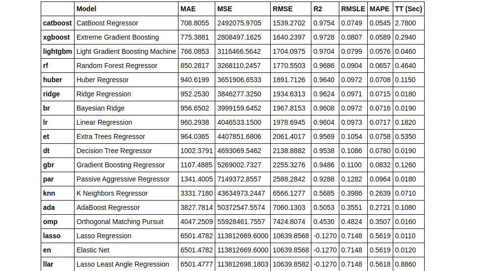
We’ve used the n_select parameter within the compare_models() to select the top 3 best performing models. By default, compare models return only the best-performing model.
type(top3)
> list
You can use print(top3) to view the models with their parameters in a list form. Since the output is really huge, I’ve not included it in this article. You can view the output in the Github repo I’ve shared at the end of the article.
In this article, we shall use a few parameters with the create_model() function.
dt = create_model('dt', fold = 5) #with 5 Fold CV

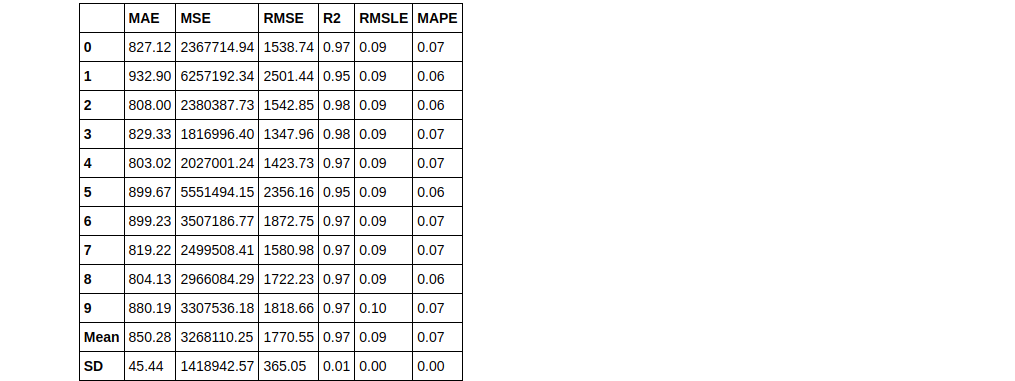
rf = create_model('rf', round = 2) #metrics rounded to 2 decimal points
Create model (KNN)
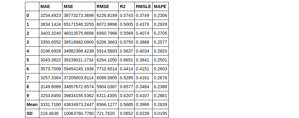
knn = create_model('knn')
tuned_knn = tune_model(knn)
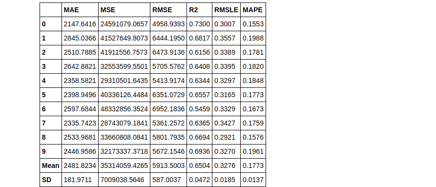
tuned_knn2 = tune_model(knn, n_iter = 50)
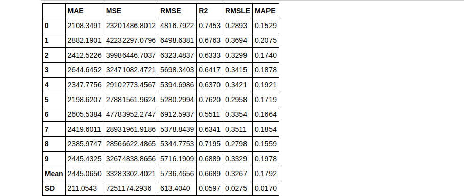
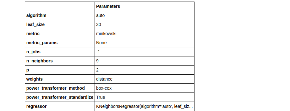
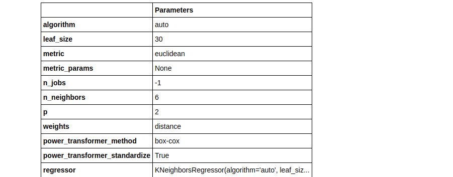
Notice how 2 tuned Knn models were built using different values of the n_iter parameter. In tuned_knn where n_iter is the default the R2 score is 0.6504 whereas, with n_iter set to 50, the R2 improved to 0.6689. Observe the differences in their hyperparameters below:
plot_model(tuned_knn, plot = 'parameter')
plot_model(tuned_knn2, plot = 'parameter')
Ensembling is a common machine learning technique used to improve the performance of tree-based models. The ensembling techniques we will cover in this article are Bagging and Boosting, using the ensemble_model() function in PyCaret.
# lets create a simple dt
dt = create_model('dt')
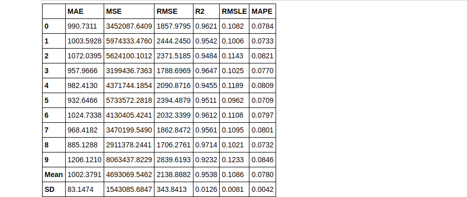
bagged_dt = ensemble_model(dt)
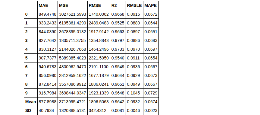
As you can see using the Bagging method we can increase the RMSLE score. Now let’s try the same with boosting.
boosted_dt = ensemble_model(dt, method = 'Boosting')
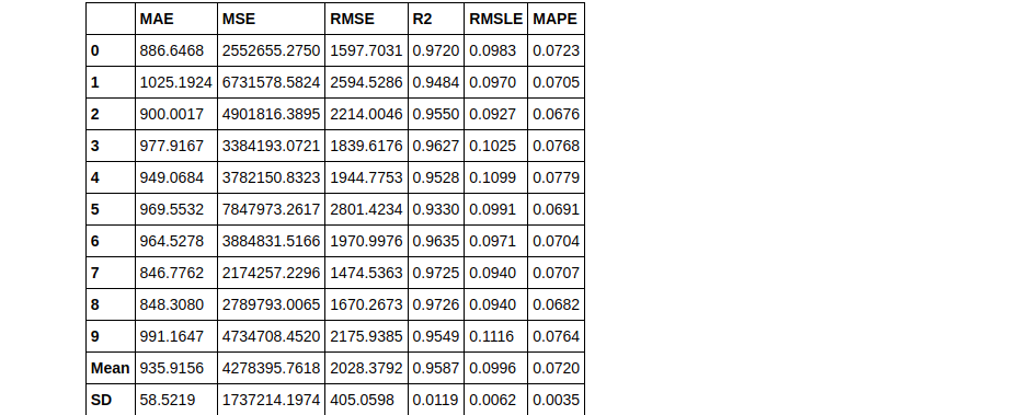
As you can see, it’s very simple to change between ensembling methods in PyCaret. Now by default, the ensemble builds 10 estimators. This can easily be changed using the n_estimators parameter. Sometimes, increasing the number of estimators can improve the results. Here’s an example:
bagged_dt2 = ensemble_model(dt, n_estimators=50)
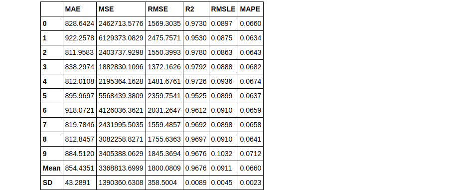
Therefore you can see that using n_estimators = 50 has yielded a better RMLSE score of 0.0911.
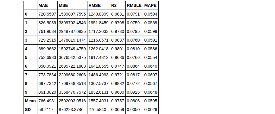
Blending creates multiple models and then averages the individual predictions to form a final prediction.
# train individual models to blend
lightgbm = create_model('lightgbm', verbose = False)
dt = create_model('dt', verbose = False)
lr = create_model('lr', verbose = False)
# blend individual models
blender = blend_models(estimator_list = [lightgbm, dt, lr])
# blend top3 models from compare_models
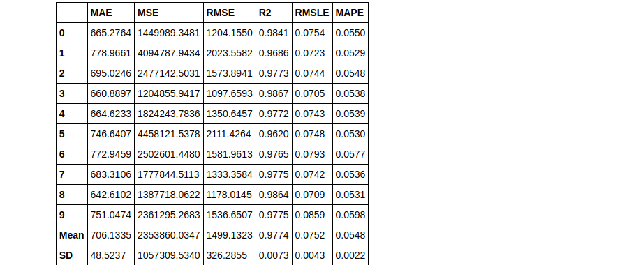
blender_top3 = blend_models(top3)
Stacking is another technique for ensembling but is not implemented as often as the others due to practical difficulties. The concept is not that hard, you can read more about stacking to get a better picture of it. Let’s see how it’s implemented in PyCaret.
We’ll use the top 3 models we got from the create_models() previously used in the article:
stacker = stack_models(top3)
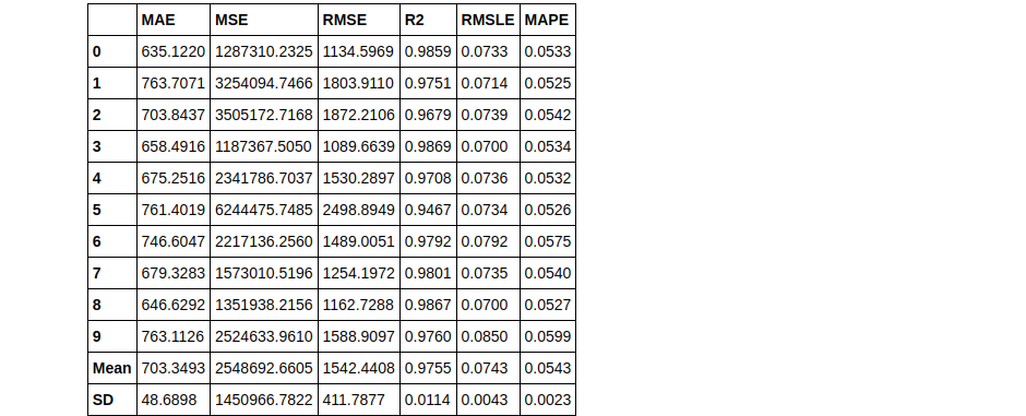
By default, the meta-model produced at the end of stacking is a Linear regression. This meta-model can easily be changed using the parameter meta_model, you can try that on your own if you want.
Many new concepts have been covered in this article. We saw how using exploratory data analysis for customizing a pipeline in setup() can help in getting more accurate results. We also learned how to perform ensembling and tune models using PyCaret.
The PyCaret series is not ending here. In my next articles, we shall see how we can perform AutoML using PyCaret for the classification problems, both binary and multiclass classifications. You can read that once it’s published, and my other articles at the following link :
Sion | Author at analytics Vidhya
If you haven’t read part 1 of the AutoML using Pycaret with a Regression Use-Case, you can read it here:
AutoML using Pycaret with a Regression Use-Case | Sion
You can connect with me on LinkedIn, or follow me on Github, where you can find the notebook for this article. Thank you for taking the time out to read my article, cheers!
The media shown in this article are not owned by Analytics Vidhya and are used at the Author’s discretion.
Lorem ipsum dolor sit amet, consectetur adipiscing elit,
Hi! I have question of this article. I am trying to get the MAE, RMSE, MSE and R2 on a model I created, but the function only give to me some metrics that are used mostly on a Classification model, not in Regression, these are Accuracy, AUC, Recall, Prec. , F1, Kappa and MCC. Do you know using which function can I get the other metrics? I have already tryed `add_metric` function, but it doesn't works. Thanks!