A Guide on Deep Learning: From Basics to Advanced Concepts

This article was published as a part of the Data Science Blogathon

Welcome to my guide! In this guide, we will cover basic as well as advanced topics involved in Deep Learning. This guide will help you in gaining confidence in the concepts of Deep Learning. So let’s begin with our journey!

Why do we need Deep Learning?

The problem 

In traditional programming, the programmer formulates rules and conditions in their code that their program can then use to predict or classify in the correct manner. For example, normally to build a classifier, a programmer comes up with a set of rules, and program those rules. Then when you want to classify things, you give it a piece of data, and rules are used to select the category. This approach might be successful for a variety of problems. But remember NOT ALL! How? Let’s see.

Image classification is one such problem that cannot be resolved using the traditional programming method. Imagine how would you write the code for image classification? How could a programmer write rules and regulations to predict images they have never seen before?

Solution Found! What is it?

Deep learning is the solution to the above problem. It is a very efficient technique in pattern recognition by trial and error. With the help of a deep neural network, we can train the network by providing a huge amount of data and providing feedback on its performance, the network can identify, through a huge amount of iteration, its own set of conditions by which it can act in the correct way.

A SIMPLE MODEL: WITH ONE NEURON

Let’s begin understanding the neural network with the simplest model that can be made. The neuron is usually represented by circles with one arrow pointing outward and one inward.

Here, in the above diagram, ‘m’ is the slope of the line, ‘x’ is the input value and ‘b’ is the constant, for the equation, y = m.x + b.

Note the difference between ‘y_hat’ and ‘y’ variables. ‘y_hat’ is the prediction that we have made using the equation called estimated value whereas ‘y’ is the actual value or true value.

Let’s see how this simple model works! We will start assigning random values to ‘m’ (usually between -1 and 1) and ‘b’, and then calculate ‘y_hat’ with the ‘x’ as input values.

In the above figure, (x, y_hat) is plotted and a regression line is drawn. Since ‘m’ and ‘b’ were given random values, there is supposed to be an error in the estimated value from the true value. Thus, the error is calculated as the average of the square of the difference between the expected value and true value i.e.

Here MSE (mean squared error) is being used but one can also use RMSE i.e. root mean squared error, which is nothing but the root of MSE.

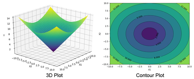
MSE basically indicates how far is the expected value from the target/ true value. If MSE is plotted on a 3D graph, it looks like the image given below:

The aim of any model is to minimize the error. Hence, the minimum of the curve is at the bottom of the curve. In order to reach there, we have to use calculus for that.  Gradient Descent is the method for finding out the minimum of this loss curve. It looks like the following graphs:

So how it works? The computer doesn’t have an eyeball like humans which does not have the ability to guestimate the path to reach the target variable from the current position. It calculates the gradient, which is the fancy word to describe multivariate slope which figures out the direction of slope, which is some ratio of the variable ‘b’ to ‘m’.

Now the direction to travel is known. The next step is to determine how far it has to travel to reach the target point. This is known as the ‘learning rate’. Usually, the learning rate is not taken to be a bigger value as it will mean that one is moving away from the target. A too-small learning rate is also a problem since it will take a longer time for computation. There are a few ways to measure the progress of the algorithm. There are epochs which mean a model update with the full dataset. Instead of epochs, nowadays people use a more efficient technique that is batch which means the sample of the full dataset. In either case, the step is either the full dataset or a batch, calculate the gradient, and update the parameters with the gradient and learning rate. Thus, the process is continued till the target value is achieved. This is how gradient descent works!

BUILDING A NETWORK: FROM NEURONS TO NETWORK

in the earlier example, only one input was considered for the neuron. Now, more inputs can be considered for one neuron. From now onwards, instead of having single x input to the neuron with slope ‘m’, multiple inputs (i.e. x1,x2,x3…so on) will be considered with their respective weights (i.e. w1, w2, w3…so on).  Not only this, there is one more interesting thing! The output of one neuron can be used as input to another neuron. This is applicable as long as it does not make a loop. When an error is calculated from new weights using gradient descent an error calculated from the later neuron can be used as part of the error of the previous neuron it’s connected to.

Gotcha! Now is the right time to introduce the concept of the Activation Function here.

ACTIVATION FUNCTIONS

There are only three types of activation functions i.e. Linear, ReLU, and Sigmoid.

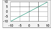
Linear Activation Function is one of the basic activation functions. This is used widely because it is fast, as it is linear in nature and hence easy to differentiate. The graph and equation of this function look like the images shown below:

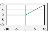
One easy way to add non linearity is to feed the equation of a line into another non-linear function. The most popular function is ReLU stands for Rectified Linear Unit. It is one of the fancy ways of saying that whenever the output of the line is negative, it is going to set it to 0. It can be represented as follows:

Another activation function is the Sigmoid function. This is an ‘S’ plot curve that goes from 0 to 1. This is the most prominent function and is widely in Logistic Regression. The result of this function gives the probability which has to lie between 0 to 1.

OVERFITTING

Why shouldn’t the programmer make a big neural network and solve every problem?  Can one think of the pitfalls of having a large model with lots of neurons?

One problem is that there will be a lot of wastage of computational resources, and the other could be the longer time to train the model. Ugh! There is one more point.

The problem is related to classical statistics. Let’s say, two models have been built, as shown below:

Which of the two models proves to be the best? One that is located on the left side. Why? look at the RMSE value. The left model has a better RMSE value than the right one. But that is not true! Why? Let’s see.

What if we get new sample data that the model has not already seen by the model? The left model would give a very poor result i.e. the RMSE will be very high as compared to the right side model. This is because the left side model has memorized the points and thus provided excellent RMSE during training. On the other hand, the right-side model is more generalized. Thus, the left hand side model is said to be the overfitted model. Thus, the choice depends on the Data Scientist to choose the type of model suitable with respect to their needs.

Now let’s create one project to understand the concepts much better :

Project Name: American Sign Language Dataset

Objectives:

1. Prepare the image data and use it for training the model

2. Create and compile the basic model for image classification

Project begins:

American Sign Language Dataset is a very common dataset and can be found on Kaggle for practice. It consists of 26 letters out of which the letters ‘j’ and ‘k’ are not considered in the training because they require movement. Their classification is beyond the scope of this guide.

Let’s start with the coding part!

Loading the Data

Reading in the Data: The sign dataset, that has been downloaded from Kaggle, is in the CSV (stands for comma-separated value) format. CSV file has rows and columns which consists of labels mentioned at the top. One can check the difference between the CSV file and XLSX file by opening them in the text (.txt) format on a usual notepad. In the CSV file, the values in a row are separated by commas.

To load and work with the data, the Pandas library would be used, which is one the best tools to work with huge data and help is easy manipulation of data. CSV files will be read in the format of Dataframe from pandas library.

import pandas as pd
train_df = pd.read_csv("sign_mnist_train.csv")
valid_df = pd.read_csv("sign_mnist_valid.csv")

Exploring the Data

Now it’s time to visualize the data. The data can be visualized by using the head method of the pandas data frame. Each row has some integer values which are nothing but the image pixel’s intensity. The data has a column labeled mentioned which refers to the true value of each image.

train_df.head()

Output:

y_valid = valid_df['label']
del train_df['label']
del valid_df['label']

x_train = train_df.values
x_valid = valid_df.values

Summarizing the Training and Validation Data

Now, the program has 27,455 images with 784 pixels each for training…

x_train.shape

…as well as their corresponding labels:

y_train.shape

For validation, it has 7,172 images…

x_valid.shape

…and their corresponding labels:

y_valid.shape

 

Visualizing the Data

To visualize the images, now use the matplotlib library. Here there is no need to worry about the details of this visualization.

Note that data will have to be reshaped from its current 1D shape of 784 pixels to a 2D shape of 28×28 pixels to make sense of the image:

mport matplotlib.pyplot as plt

plt.figure(figsize=(40,40))

​num_images = 20

for i in range(num_images):

    row = x_train[i]

    label = y_train[i]

    image = row.reshape(28,28)

    plt.subplot(1, num_images, i+1)

    plt.title(label, fontdict={'fontsize': 30})

    plt.axis('off')

    plt.imshow(image, cmap='gray')

Normalize the Image Data

Deep learning models are much better and very efficient at dealing with floating-point numbers between 0 and 1. The Conversion of integer values to floating-point values between 0 and 1 is called normalization. Normalization is a very essential concept that one should be aware of.

Now it’s time to normalize the image data, meaning that their pixel values, instead of being between 0 and 255 as they are currently:

x_train.min()

x_train.max()

…should be floating-point values between 0 and 1. It is coded as follows:

x_train = x_train / 255
x_valid = x_valid / 255

Categorize the Labels

What is categorical encoding?

Consider the case, if someone asks, what is 7-2? If you said that digit 4 is much closer to the answer than digit 9. Unfortunately, this does not happen in neural networks used for image classification. The neural networks should not have this kind of reasoning and it should clearly make a difference that guessing the image as 4, which is actually 5, is equivalently bad as guessing 9.

We can see that images are labeled between 0 to 9. Since these are numerical values, the model thus created should try to categorize them perfectly into ten categories.

Since it was previously mentioned that labels are values, it is required for them to get converted into categories. For this, category encoding is used, which modifies the data so that each label belongs to its possible category. The keras.utils.to_categorical method will be used to accomplish this.

import tensorflow.keras as keras
num_classes = 24
y_train = keras.utils.to_categorical(y_train, num_classes)
y_valid = keras.utils.to_categorical(y_valid, num_classes)

Build the Model

The data is all prepared, we have normalized images for training and validation, as well as categorically encoded labels for training and validation.

With the training data that we prepared earlier, it is now time to create the model that will train with the data. This first basic model will be made up of several layers and will be comprised of 3 main parts:

1. An input layer, the layer which receives all data as input
2. Several hidden layers, each made up of many neurons. Each neuron will have its weight associated with it such that it will affect the performance and accuracy of the model.
3. An output layer, which will depict the network’s guess for a given image

The units argument specifies the number of neurons in the layer. The activation function concept has already been taught above.

from tensorflow.keras.models import Sequential
from tensorflow.keras.layers import Dense
model = Sequential()
model.add(Dense(units = 512, activation='relu', input_shape=(784,)))
model.add(Dense(units = 512, activation='relu'))
model.add(Dense(units = num_classes, activation='softmax'))

Summarizing the Model

The below code will give the way to summarize the model:

model.summary()

Compiling the Model

Time to compile our model with the same options, using categorical cross-entropy to ensure that we want to fit into one of many categories, and measure the accuracy of our model:

model.compile(loss='categorical_crossentropy', metrics=['accuracy'])

Train the Model

Use the model’s fit method to train it for 20 epochs using the training and validation images and labels created above:

model.fit(x_train, y_train, epochs=20, verbose=1, validation_data=(x_valid, y_valid))

Now one can see the training of the model for 20 epochs. The accuracy turns out to be 97% approximately which is quite good.

So, this was all about Deep learning techniques. I hope you enjoyed the guide and have been able to give a head start with deep learning.

All the best! Stay tuned for more articles and guide on Analytics Vidhya!

Want to read more about Deep Learning? Click here!

The media shown in this article is not owned by Analytics Vidhya and are used at the Author’s discretion. 

Sarvagya 29 Dec, 2021

Hi, I'm Sarvagya Agrawal, Software Engineer, with a strong passion for utilizing technology to drive positive change in society. I believe that technology is not just a skill, but an art form that can be leveraged to transform the world. My primary focus lies in machine learning and web development, with strong programming skills in Python. I have worked on innovative projects, including developing an AI model to calculate cardiovascular risk factors from OCTA scans using computer vision algorithms and creating an AI-based web application for calculating financial risk based on an individual's spending trends.