In this article, we will distinguish between various tree-based machine learning algorithms, focusing on their complexity and practical applications. Tree-based models, including Classification and Regression Trees (CART), are a subset of supervised machine learning methods. They perform classification and regression tasks by constructing a tree-like structure to determine the target variable class or value based on input features.
Tree-based algorithms are widely popular for predicting outcomes in both tabular and spatial/GIS datasets. Our discussion will cover four levels of tree-based machine learning algorithms, ranging from the simplest to the most complex.
This article was published as a part of the Data Science Blogathon.
A tree-based model starts with a root node and branches out into multiple levels, forming a tree-like structure. Each internal node represents a decision based on a feature, each branch represents the outcome of the decision, and each leaf node represents a final prediction. At each depth level, conditions based on feature values determine the direction of the branches. The process continues until a leaf node is reached, providing the final prediction.
Example: Simple Decision Tree
Let’s consider a simple decision tree created to predict the most suitable water resource for a location. The features include:
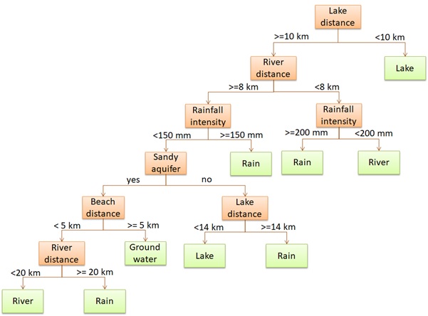
The decision tree helps determine whether the community should utilize rainfall, river water, lake water, or groundwater based on these features.
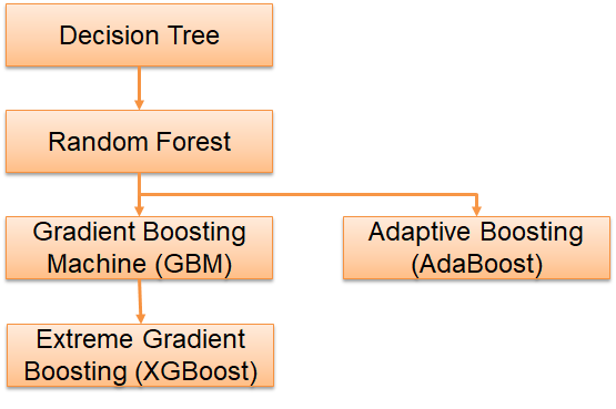
Let’s start with the simplest tree-based algorithm. It is the Decision Tree Classifier and Regressor. Actually, we have discussed the Decision Tree in the second and third paragraphs. A single Decision Tree is created by fitting training data. Imagine we asked a robot to learn from 10,000 training data and later we want the robot to predict the other 20,000 test data for us. We can feel that only one piece of feedback is not enough. We need more robots to learn the training data and do more predictions for us.
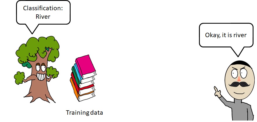
The decision tree algorithm segments a dataset into distinct classes through a series of binary decisions. Let’s illustrate this with an example of segmenting data points into two classes: “sold out” and “not sold out.”
First, the algorithm starts by dividing the data based on one of the features. For instance, it might split the data on the price feature at $600. This creates two groups: products priced above $600 and products priced below $600.
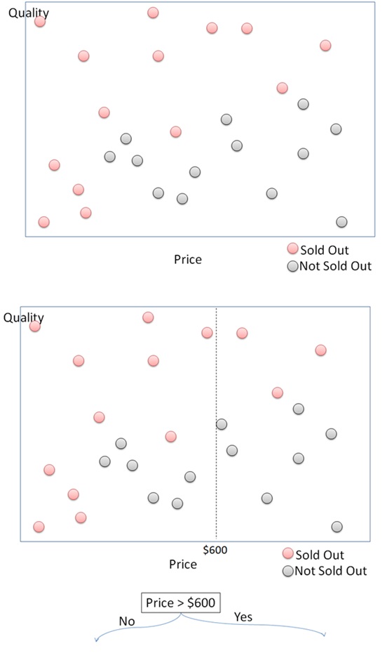
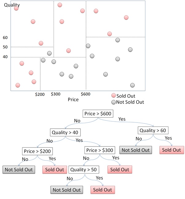
Next, for products priced above $600, the algorithm then checks the quality feature. If the quality is above 60, the products are likely to be sold out. Otherwise, they are not sold out. For products priced below $600, the algorithm continues to split further. It might check other features such as price ranges or quality levels to refine the segmentation.
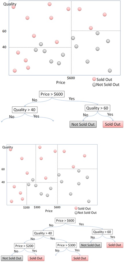
Each decision at a node splits the dataset into smaller subsets. This process continues recursively, creating a tree structure where each node represents a decision based on a feature. The process continues until it reaches the terminal nodes or leaves, which represent the final class prediction. Each path from the root to a leaf represents a series of decisions that classify the data point.
Let’s take it to the next level with the Ensemble Method. This approach uses multiple models to improve accuracy and reliability. By applying different algorithms like Decision Trees, Support Vector Machines, Neural Networks, kNN, and Naive Bayes to the same training dataset, we can build several models. For example, with five models, we predict the test dataset and decide the final output through majority voting for classification or averaging for regression.
One of the most popular ensemble methods is the Random Forest. It combines multiple decision trees to make predictions. This involves training several decision trees on different subsets of the data and then combining their predictions. This approach significantly improves performance, making the results more accurate and reliable compared to using a single model.
In a Random Forest, multiple decision trees are built using different subsets of the training dataset. This technique, known as Bagging (Bootstrap Aggregating), ensures that each tree learns from different aspects of the data, enhancing the overall prediction. For example, we might train five decision trees on different subsamples of the data. Each tree makes its prediction independently, and the final prediction is determined by majority voting for classification or averaging for regression.
Classification
Suppose we have five decision trees predicting whether a location should use “Rain” or “River” as a water resource. If four trees vote for “River” and one votes for “Rain”, the Random Forest will predict “River”.

Regression
For regression tasks, each tree provides a numerical prediction. The final output is the average of these predictions. For example, if five trees predict values of 18, 8, 16, 15, and 10, the final prediction is the average: (18 + 8 + 16 + 15 + 10) / 5 = 13.4.

While Bagging (Bootstrap Aggregating) or Random Forest involves training multiple models independently and simultaneously, Boosting takes a different approach to enhance model accuracy. In Boosting, models are created sequentially, with each new model learning from the mistakes of the previous ones.
Boosting Process:
This iterative process continues until a specified number of models are built. By allowing each base model to learn from the errors of its predecessor, Boosting can achieve higher accuracy. It transforms individual weak learners into a robust ensemble, similar to how a team of cooperating robots can achieve more together than they could individually.

Two of the most popular boosting algorithms are AdaBoost and Gradient Boosting. Both techniques aim to reduce bias and variance, but they do so in different ways.
AdaBoost works by sequentially applying a weak learner to modified versions of the data. It starts by training the weak learner on the entire dataset and then adjusts the weights of the incorrectly classified instances, making them more important in the next iteration. This process is repeated multiple times, each time focusing more on the errors made by the previous weak learner. The final model is a weighted sum of the weak learners, where the weights depend on the performance of each weak learner.
Gradient Boosting builds the model in a stage-wise manner, much like AdaBoost, but it focuses on optimizing a loss function. Each new weak learner is trained to correct the errors made by the previous learners. Specifically, it fits the new learner to the negative gradient of the loss function, which represents the errors of the current model. This approach allows Gradient Boosting to handle various loss functions and be more flexible than AdaBoost.
XGBoost, short for Extreme Gradient Boosting, is an advanced implementation of the Gradient Boosting algorithm designed for speed and performance. It has become a popular choice for winning machine learning competitions and is known for its robustness and scalability. XGBoost includes several enhancements over traditional Gradient Boosting, making it a powerful tool for both regression and classification tasks.
| Algorithm | Description | Advantages | Disadvantages | Typical Applications |
|---|---|---|---|---|
| Decision Trees | Simple tree structure for classification and regression tasks. | – No need for feature scaling – Handles both numerical and categorical data – Simple to understand and interpret | – Prone to overfitting – Less accurate compared to ensemble methods | Basic classification and regression |
| Random Forests | Ensemble method using multiple decision trees (Bagging) to improve accuracy and control overfitting. | – Reduces overfitting – Handles large datasets – Improves prediction accuracy | – Computationally intensive – Less interpretable than single decision trees | Complex classification and regression tasks, especially with large datasets |
| AdaBoost | Boosting technique where each new model focuses on correcting the errors of the previous ones. | – Reduces bias and variance – Improves accuracy sequentially | – Sensitive to noisy data and outliers – More complex to implement and interpret | Applications requiring high accuracy, dealing with imbalanced datasets |
| Gradient Boosting (GBM) | Boosting method focusing on optimizing a loss function through stage-wise additions of weak learners. | – Handles various loss functions – High accuracy and flexibility | – Prone to overfitting if not properly regularized – Requires careful tuning | High-accuracy prediction tasks, both classification and regression |
| XGBoost | Advanced implementation of Gradient Boosting with enhancements for speed and performance. | – Regularization to prevent overfitting – Handles missing data – Parallel processing – Tree pruning and shrinkage for robust learning | – Complex to implement – Requires significant computational resources | Winning machine learning competitions, large-scale predictive modeling |
Also Read:
This article distinguishes tree-based Machine Learning into 4 complexity levels. The simplest model is the Decision Tree. A combination of Decision Trees builds a Random Forest. Random Forest usually has higher accuracy than Decision Tree does. A group of Decision Trees built one after another by learning their predecessor is Adaptive Boosting and Gradient Boosting Machine.
Adaptive and Gradient Boosting Machine can perform with better accuracy than Random Forest can. Extreme Gradient Boosting is created to compensate for the overfitting problem of Gradient Boosting. Thus, we can say that in general Extreme Gradient Boosting has the best accuracy amongst tree-based algorithms. Many say that Extreme Gradient Boosting wins many Machine Learning competitions. If you find this article useful, please feel free to share.
Want to become a Data Scientist? Enroll in our AI/ML BlackBelt Plus program and learn all the skills required to become a leading Data Scientist!
A. Tree-based machine learning models are supervised learning methods that use a tree-like model of decision making to perform classification and regression tasks. They include algorithms like Classification and Regression Trees (CART), Random Forests, and Gradient Boosting Machines (GBM). These algorithms handle both numerical and categorical variables and can be implemented in Python using libraries like scikit-learn.
A. Decision tree models segment a dataset into distinct classes through a series of binary decisions based on input variables. Each split in the tree is based on metrics like entropy or the gini index to measure impurity, determining how well a split separates the data. The tree continues to split until it reaches leaf nodes, which represent the final prediction. Information gain, calculated using entropy, helps in selecting the best splits to improve prediction accuracy.
A. Tree-based models have several advantages, including:
– No need for feature scaling, unlike linear regression and logistic regression.
– Ability to handle both numerical and categorical data.
– Capability to capture non-linear relationships.
– Flexibility to be combined into ensemble learning methods like Random Forests and Boosting techniques for enhanced predictive power and robustness.
A. Ensemble learning in Random Forests involves building multiple decision tree models using different subsets of the training data. This technique, known as Bagging (Bootstrap Aggregating), reduces overfitting and improves prediction accuracy by averaging the results (regression problems) or using majority voting (classification tasks). Random Forests are particularly effective with large datasets and diverse predictors.
A. XGBoost is an advanced implementation of Gradient Boosting (GBM) designed for speed and performance optimization. It includes features like regularization (to control model complexity and prevent overfitting), handling of missing data, parallel processing, and tree pruning. XGBoost’s use of shrinkage (learning rate) and built-in cross-validation ensures robust learning and better performance on unseen data compared to traditional GBM methods.
The media shown in this article are not owned by Analytics Vidhya and is used at the Author’s discretion.
Lorem ipsum dolor sit amet, consectetur adipiscing elit,